
Among the myriad of machine learning algorithms and techniques available with data scientists, one stands out for its exceptional performance in classification problems: XGBoost, short for eXtreme Gradient Boosting. This algorithm has established itself as a force to reckon with in the data science community, as evidenced by its frequent use and high placements in Kaggle competitions, a platform where data scientists and machine learning practitioners worldwide compete to solve complex data problems. The following plot is taken from Francois Chollet tweet.
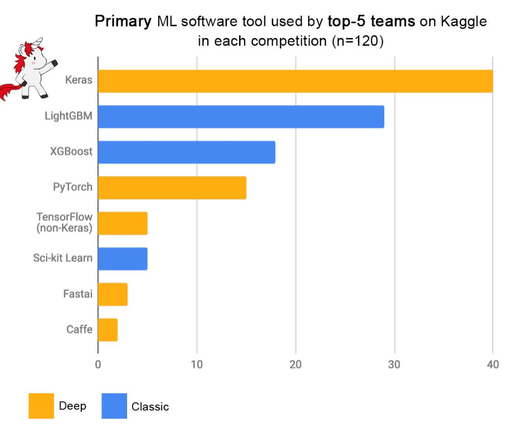
Above demonstrates the prominence of XGBoost as one of the primary machine learning software tools used by the top-5 teams across 120 Kaggle competitions. The data points in the plot showcase that XGBoost is one of the most preferred choices, surpassing even deep learning giants like TensorFlow and PyTorch in certain contexts.
In this blog, we will delve into the workings of the XGBoost classifier, unpacking its fundamentals and demonstrating its implementation with a Python example using the well-known Iris dataset. Whether you are a beginner looking to understand the basics or an experienced data scientist seeking to refine your toolkit, this walkthrough will provide you with a practical understanding of how XGBoost can be leveraged to solve classification challenges efficiently and with high accuracy.
What is XGBoost Classifier?
XGBoost is an advanced implementation of gradient boosting algorithms, widely used for training machine learning models. It’s designed to be highly efficient, flexible, and portable. At its core, XGBoost is a decision-tree-based ensemble machine learning algorithm that uses a gradient boosting framework. Gradient boosting is the backbone of XGBoost. It’s a technique of converting weak learners (simple decision trees) into strong learners in a sequential manner.
The XGBoost classifier operates by sequentially adding predictors (decision trees) to an ensemble, each one correcting its predecessor. Decision trees are the fundamental building blocks of an XGBoost model. Each tree in the ensemble is constructed to predict the residuals (errors) left over by the previous trees. Essentially, every new tree is learning from the mistakes of its predecessors, improving the model’s accuracy with each step. The use of multiple shallow trees, as opposed to a single deep tree, helps in reducing overfitting.
How does XGBoost Classifier work?
The following is the step-by-step functioning of how XGBoost classifier, or for that matter, XGBoost, works:
- Initialization: The algorithm begins with a simple model. This initial model could be as basic as a single decision tree or even a constant value that predicts the average outcome of the dataset. This model provides the first set of predictions.
- Computing the Residuals: The algorithm calculates the residuals or errors of these initial predictions. These residuals are simply the differences between the predicted values and the actual values of the target variable.
- Building Trees to Correct Errors: For each subsequent step, XGBoost constructs a new decision tree that aims to predict these residuals. The idea is to gradually improve the predictions by focusing on where the previous model performed poorly.
- Gradient Descent Optimization: At each step, the algorithm applies gradient descent to minimize the loss function, which is a measure of the difference between the predicted outcomes and the actual outcomes. This involves updating the model in the direction that reduces the loss.
- Updating the Model: After building each tree, the model gets updated to include the new tree. Rather than simply adding the tree’s predictions, the model scales these predictions by a factor known as the learning rate. This rate helps to control the model’s learning speed and prevents overfitting.
- Regularization: XGBoost includes a regularization term in its objective function, which controls the complexity of the model. This is crucial for avoiding overfitting, especially when dealing with noisy datasets.
- Iterative Learning: The process of adding trees continues iteratively. Each new tree is built to correct the residual errors made by the combined predictions of all previous trees. The algorithm stops adding trees when it reaches a specified maximum number of trees or when additional trees fail to meaningfully reduce the loss function.
- Output: The final model is an ensemble of many decision trees. To make a prediction, XGBoost sums the predictions from all individual trees. This ensemble approach allows the model to capture complex patterns in the data, leading to high predictive accuracy.
Why use XGBoost Classifier?
XGBoost has become a go-to algorithm for many data scientists for classification tasks, and its popularity is grounded in several compelling reasons. Here are the top three reasons why XGBoost can often be the preferred choice for classification problems:
- Performance and Accuracy: XGBoost is designed to optimize computational efficiency and memory usage, which translates into fast execution speeds. It uses advanced techniques such as gradient boosting, which allows for more accurate models by focusing on correcting the mistakes of previous trees in the sequence. Additionally, it has built-in regularization which helps to prevent overfitting, resulting in better generalization on unseen data.
- Versatility in Handling Various Types of Data: XGBoost can handle a wide range of data formats including CSV, NumPy arrays, and Pandas data frames. It can also accommodate both continuous and categorical variables. The algorithm is robust to missing data and various data scales, which eliminates the need for extensive data preprocessing like normalization or imputation.
- Flexibility and Fine-Tuning: XGBoost provides a plethora of hyperparameters that can be fine-tuned to improve the model’s performance. This includes the depth of the trees, learning rate, and many others which allow the model to be very sensitive to the specific patterns in the data. It also supports various objective functions and evaluation criteria, making it highly adaptable to the specific needs of a wide array of classification problems.
XGBoost Classifier Python Example
In this section, we will learn how to train an XGBoost classifier using Python’s XGBoost library in conjunction with the Scikit-learn framework. Sklearn modules are used for data processing, model building, and evaluation. The XGBoost library in Python integrates smoothly with Sklearn, allowing for a familiar and accessible experience for those already comfortable with Sklearn’s workflow.
Step #1: Setting Up the Environment
Before diving into the example, ensure that you have the necessary libraries installed. If not, you can install them using pip:
pip install xgboost
pip install scikit-learn
Step #2: Dataset and Preprocessing
For this example, let’s use the famous Iris dataset, which is a simple yet effective dataset for classification tasks.
from sklearn.datasets import load_iris
from sklearn.model_selection import train_test_split
from sklearn.preprocessing import LabelEncoder

# Load dataset
iris = load_iris()
X = iris.data
y = iris.target

# Split the dataset into train and test sets
X_train, X_test, y_train, y_test = train_test_split(X, y, test_size=0.3, random_state=42)
Step #3: Training & testing XGBoost Classifier
Now, let’s implement the XGBoost classifier. We’ll use the XGBClassifier from the XGBoost package, which is designed to work seamlessly with Sklearn.
from xgboost import XGBClassifier
from sklearn.metrics import accuracy_score

# Initialize the XGBClassifier
xgb_clf = XGBClassifier()

# Fit the classifier to the training data
xgb_clf.fit(X_train, y_train)

# Predict the labels of the test set
y_pred = xgb_clf.predict(X_test)

# Evaluate the classifier
accuracy = accuracy_score(y_test, y_pred)
print(f"Accuracy: {accuracy:.2f}")
Step #4: Hyperparameter tuning of XGBoost Classifier
XGBoost offers a variety of parameters that can be tuned to improve performance. Some of the key parameters include:
- learning_rate: Step size shrinkage used to prevent overfitting. Range is [0,1]
- max_depth: Maximum depth of a tree. Increasing this value will make the model more complex and more likely to overfit.
- n_estimators: Number of trees you want to build.
- objective: Specifies the learning task and the corresponding learning objective. For example, binary:logistic for binary classification.
# Example of a customized XGBoost classifier
custom_xgb_clf = XGBClassifier(n_estimators=100, learning_rate=0.1, max_depth=5)
custom_xgb_clf.fit(X_train, y_train)
custom_y_pred = custom_xgb_clf.predict(X_test)
custom_accuracy = accuracy_score(y_test, custom_y_pred)
print(f"Custom Model Accuracy: {custom_accuracy:.2f}")

Check out my latest book titled as First Principles Thinking: Building winning products using first principles thinking.
- Mathematics Topics for Machine Learning Beginners - July 6, 2025
- Questions to Ask When Thinking Like a Product Leader - July 3, 2025
- Three Approaches to Creating AI Agents: Code Examples - June 27, 2025
I found it very helpful. However the differences are not too understandable for me