While training machine learning models, we come across the need for scaling features in order to have different features contribute to the predictions in an appropriate manner. Without scaling, features with larger numerical ranges can dominate those with smaller ranges, leading to biased or inefficient learning. In this post you will learn about this feature engineering technique namely feature scaling with Python code examples using which you could significantly improve performance of machine learning models. To demonstrate the technique, the models will be trained using Perceptron (single-layer neural network) classifier.
What is Feature Scaling? Why is it needed?
Feature scaling is a method used to standardize the range of independent variables or features of data. In data processing, it is also known as data normalization or standardization. Feature scaling is generally performed during the data pre-processing stage, before training models using machine learning algorithms. The goal is to transform the data so that each feature is in the same range (e.g. between -1 to 1 or 0 to 1). This ensures that no single feature dominates the others, and makes training and tuning quicker and more effective.
Feature scaling can be accomplished using a variety of linear and non-linear methods, including min-max scaling, z-score standardization, clipping, winsorizing, taking logarithm of inputs before scaling, etc. Which method you choose will depend on your data and your machine learning algorithm.
To understand the feature scaling concept with an example, consider a dataset with two features, age and salary. Age is usually distributed between 0 and 80 years, while salary is usually distributed between 0 and 1 million dollars. If we apply linear regression algorithm to this dataset without feature scaling, the algorithm will give more weight to the salary feature since it has a much larger range. However, by rescaling both features to the range [-1, 1], we can give both features equal weight and improve the performance of our machine learning algorithm.
Why feature scaling is needed in the first place?
Machine learning algorithms using optimizing or learning algorithms such as gradient descent optimizers which are tuned to work well with numbers in the [-1, 1] range, require scaling the numeric values to lie in that range. The primary reason is the following:
Optimization algorithms such as Gradient descent require more steps to converge with larger magnitudes as the curvature of the loss function increases. The reason is that the derivatives of features with larger relative magnitudes will tend to be larger as well, and this will result in abnormal and undesirable weight updates. For larger weight updates, it will require more steps to converge and thereby increase the computation load.
Scaling the data such that it lies in the range [–1, 1] would make the error function more spherical. Thus, models trained with transformed / scaled data in the range of [-1, 1] will tend to converge faster and are therefore faster/cheaper to train. In addition, the [–1, 1] range offers the highest floating point precision. The following code can be run to check the computation time it takes to train model with raw data and the training data:
import timeit
from sklearn import datasets, linear_model
#
# Load the Sklearn diabetes data set
#
diabetes_X, diabetes_y = datasets.load_diabetes(return_X_y=True)
#
# Create scaled data set
#
raw = diabetes_X[:, None, 2]
max_raw = max(raw)
min_raw = min(raw)
scaled = (2*raw - max_raw - min_raw)/(max_raw - min_raw)
#
# Define method for training a linear regression model with
# raw and scaled data set
#
def train_raw_data():
    linear_model.LinearRegression().fit(raw, diabetes_y)
def train_scaled_data():
    linear_model.LinearRegression().fit(scaled, diabetes_y)
#
# Use the timeit method to measure the
# execution of training method
#
raw_time = timeit.timeit(train_raw_data, number=1000)
scaled_time = timeit.timeit(train_scaled_data, number=1000)
#
# Print the time taken to
# train the model with raw data and scaled data
#
raw_time, scaled_time
Another reason why one must go for scaling dataset is that some machine learning algorithms and techniques are very sensitive to the relative magnitudes of the different features. For instance, the clustering algorithm such as k-means uses the Euclidean distance as its proximity measure. This will result in algorithm rely heavily on features with relatively larger magnitudes.
Yet another reason why one must go for feature scaling is that the lack of scaling affects the efficacy of L1 or L2 regularization since the magnitude of weights for a feature depends on the magnitude of values of that feature, and so different features will be affected differently by regularization. By scaling all features to lie between [–1, 1], it can be ensured that there is not much of a difference in the relative magnitudes of different features.
How do we scale the features?
There are different techniques which can be followed to scale the feature before you use the data for training your models. These techniques include min-max scaling and Z-score normalization (also known as standard scaling).
Different types of features scaling
Feature scaling is performed when the dataset contains features that are highly varying in magnitudes, units, and ranges. The following is the details related to different kind of scaling as briefed above:
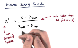
- Min-max scaling: Min-max scaling method is used to standardize data and ensure that all features are on a similar scale ([0, 1]). It makes training the model more efficient. For example, imagine we are training a model to predict house prices. If one of the features is the size of the house in square feet, we would want to make sure that this value is scaled appropriately before feeding it into the model. Otherwise, the model may place too much importance on this feature and produce inaccurate predictions. Min-max scaling can be used to achieve this goal by transforming all values so that they fall within a specific range (e.g., [0,1]). The following is the formula for min-max scaling:
x_scaled = (x1 -x1_min)/(x1_max – x1_min)
The problem with min-max scaling is that the maximum and minimum value (x1_max and x1_min) would need to be estimated from the training dataset, and they often turn out to be outlier values. Thus, the real data often gets shrunk to a very narrow range in the [0, 1] band.
The following plots demonstrate the effect of min-max scaling on a dataset with two features. In the left plot, you can see that the scale of Feature 2 is much larger than that of Feature 1. This disparity in scale can lead to issues in machine learning models, as models might incorrectly interpret the feature with the larger scale as being more important. In the right plot, both features have been scaled to fit within the range of [0, 1]. This normalization ensures that each feature contributes approximately equally to the model’s predictions, improving the performance and stability of machine learning algorithms.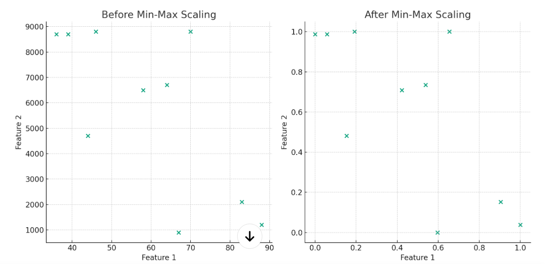
In Python, this can be implemented easily using libraries like Scikit-learn with MinMaxScaler (sklearn.preprocessing.MinMaxScaler).
import numpy as np
from sklearn.preprocessing import MinMaxScaler
#Example data
data = np.array([[1, 2, 3], [4, 5, 6], [7, 8, 9]])
#Create the scaler and scale the data
scaler = MinMaxScaler()
scaled_data = scaler.fit_transform(data)
#Display the scaled data
print(scaled_data) - Z-score normalization: Z-score normalization, also known as Z-score standardization or mean-variance scaling, is a method of feature scaling that aims to rescale features in the range of [-1, 1] so that they have a mean of zero and a standard deviation of one. It addresses the problem of outliers without requiring prior knowledge of what the reasonable range is by linearly scaling the input using the mean and standard deviation estimated over the training dataset.
The following plots illustrate the effect of standard scaling (Z-score normalization) on the same dataset. In the left plot, similar to the min-max scaling example, you can observe the disparity in scale between Feature 1 and Feature 2. In the right plot, the data is transformed such that each feature now has a mean of 0 and a standard deviation of 1.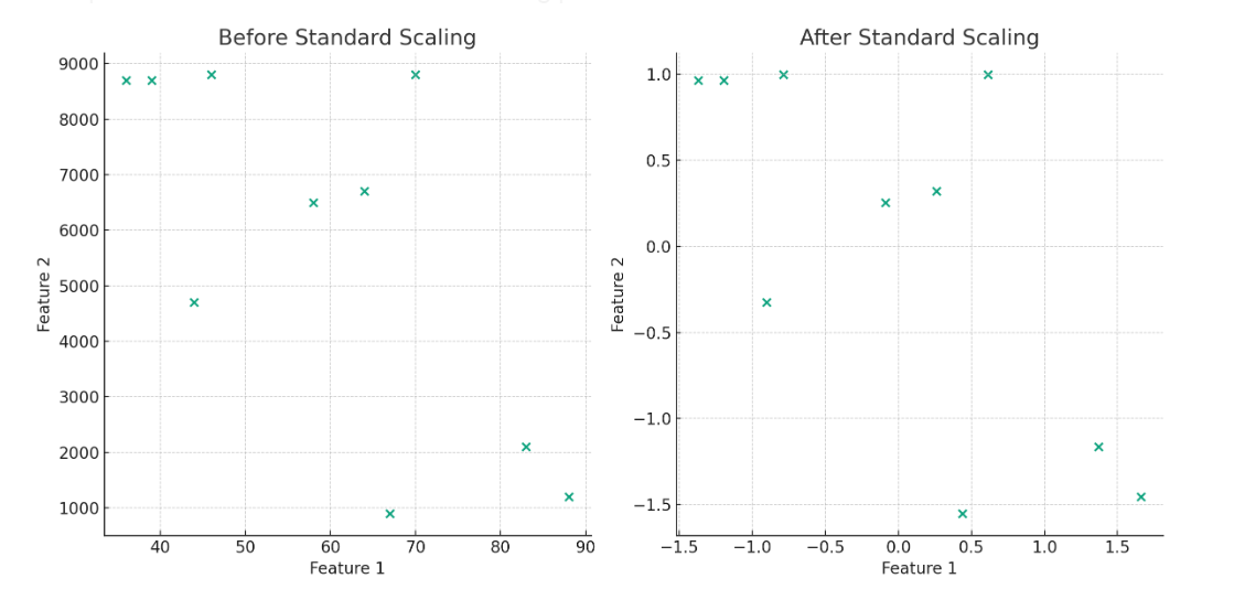
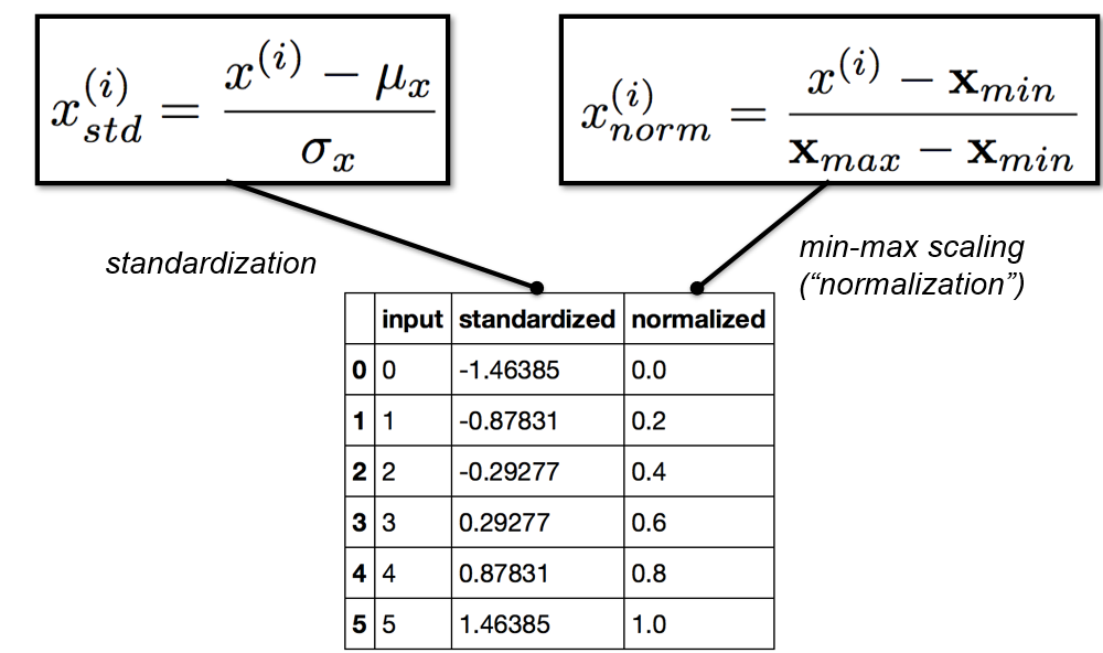
Z-score normalization is most effective when the data is normally distributed. When Z-score normalization is applied to non normal datasets, it may compress some of the data points and expand others, which can impact the models’ accuracy. The following represents the formula for Z-score normalization. The same is implemented in StandardScaler (sklearn.preprocessing.StandardScaler) whose usage is shown later in this post.x_scaled = (x1 – x1_mean)/x1_stddev
The picture below represents the formula for both standardization and min-max scaling.
import numpy as np
from sklearn.preprocessing import StandardScaler

# Example data
data = np.array([[1, 2, 3], [4, 5, 6], [7, 8, 9]])

# Create the scaler and scale the data
scaler = StandardScaler()
scaled_data = scaler.fit_transform(data)

# Display the scaled data
print(scaled_data)
- Logarithmic Scaling: Logarithmic scaling, commonly known as log scaling, is another technique that involves applying the logarithmic function to each data point, transforming the data to a logarithmic scale. This method is particularly effective when dealing with data that has a skewed distribution, as it helps in reducing the effect of outliers and extreme values. By compressing the range of large values and expanding the range of small values, log scaling makes the data more manageable and suitable for algorithms that assume a normal distribution.
The formula of log scaling involves applying a logarithmic function to each data point in a dataset. The general form of this transformation is expressed as:
$y_i = \log_b(x_i + c)$
Where $y_i$ is the transformed value, $x_i$ is the original value, c is a constant added to each data point before applying the logarithm, often used to avoid the issue of taking the logarithm of zero or negative numbers. - Winsorizing / Clipping: Winsorizing, also termed as feature clipping, is a method used to limit the extreme values in a dataset to reduce the impact of outliers. Essentially, it involves setting all data points that are below a certain percentile (e.g., the 5th percentile or the 10th percentile) to the value at that percentile, and setting all data points above another percentile (e.g., the 95th percentile or the 90th percentile) to the value at that percentile. Winsorizing ensures that outliers do not have an inordinate influence on statistical results by capping them to a certain range. It’s a compromise between keeping the data intact and completely removing outliers. This technique is particularly useful when the nature of the data is such that it can have extreme values that are legitimate observations, but may distort statistical analyses.
import numpy as np
from scipy.stats import mstats
data = np.array([1, 2, 3, 4, 5, 6, 7, 8, 9, 10, 15, 25, 30, 100, 101, 102, 103, 108, 109, 112, 115, 125])
# Winsorizing at the 10% and 90% percentiles
winsorized_data = mstats.winsorize(data, limits=[0.1, 0.1])
print(winsorized_data)
The following gets printed. Note the winsorized data in the beginning and end of the array.
[ 3 3 3 4 5 6 7 8 9 10 15 25 30 100 101 102 103 108 109 112 112 112]
Non-linear transformation: Consider the scenario when the training data is found to be skewed and neither uniformly or normally distributed? In that case, it is recommended to apply non-linear transformation to the training data before going for scaling it. One of the most common trick is to take the logarithm of the training data and then apply one of the scaling techniques as discussed above. Other common non-linear transformations techniques include taking the sigmoid and polynomial expansions (square, square root, cube, cube root, and so on) before applying the scaling techniques.
Example Scenario: Train a Model with Feature Scaling
In this section, we will look at the end-to-end flow of training a Perceptron model while doing feature scaling. We can see a significant improvement in the performance of models when features are scaled using appropriate method discussed above.
from sklearn.preprocessing import StandardScaler
sc = StandardScaler()
sc.fit(X_train)
X_train_std = sc.transform(X_train)
X_test_std = sc.transform(X_test)
The above code represents StandardScaler class of sklearn.preprocessing module. The fit method of StandardScaler is used to estimate sample mean and standard deviation for each feature using training data. The transform method is then used to estimate the standardized value of features using those estimated parameters (mean & standard deviation).
The next step is to train a Perceptron model and measure the accuracy:
prcptrnFS = Perceptron(eta0=0.1, random_state=1)
prcptrnFS.fit(X_train_std, Y_train)
Y_predict_std = prcptrnFS.predict(X_test_std)
print("Misclassified examples %d" %(Y_test != Y_predict_std).sum())
from sklearn.metrics import accuracy_score
print("Accuracy Score %0.3f" % accuracy_score(Y_test, Y_predict_std))
The accuracy score comes out to be 0.978 with the number of misclassified examples as 1. You can note that the accuracy score increased by almost 40%. Thus, it is recommended to perform do feature scaling before training the model.
Conclusion
That’s all for now. I hope you found this article helpful. If you have any questions, please don’t hesitate to let me know. I would also be happy to provide more information on linear and non-linear feature transformation feature scaling techniques such as min-max scaling, Z-score normalization, logarithmic transformation, etc. of training data if you are interested.

Check out my latest book titled as First Principles Thinking: Building winning products using first principles thinking.
- Mathematics Topics for Machine Learning Beginners - July 6, 2025
- Questions to Ask When Thinking Like a Product Leader - July 3, 2025
- Three Approaches to Creating AI Agents: Code Examples - June 27, 2025
I found it very helpful. However the differences are not too understandable for me