Last updated: 24th Nov, 2023
Dimensionality reduction is an important technique in data analysis and machine learning that allows us to reduce the number of variables in a dataset while retaining the most important information. By reducing the number of variables, we can simplify the problem, improve computational efficiency, and avoid overfitting.
Principal Component Analysis (PCA) is a popular dimensionality reduction technique that aims to transform a high-dimensional dataset into a lower-dimensional space while retaining most of the information. PCA works by identifying the directions that capture the most variation in the data and projecting the data onto those directions, which are called principal components.
However, when we apply PCA, it is often important to understand how much of the variation in the data is explained by each principal component. This is where the concept of “explained variance” comes in. Explained variance measures the proportion of variance in the data that is explained by each principal component.
In this blog post, you will learn about the concepts of explained variance which is one of the key concepts related to principal component analysis (PCA). The explained variance concepts will be illustrated with Python code examples. We will provide a detailed technical explanation of the underlying concepts of PCA, as well as practical examples of how to implement PCA and calculate explained variance using Python. Check out the concepts of Eigenvalues and Eigenvectors in this post – Why & when to use Eigenvalue and Eigenvectors.
What is Explained Variance?
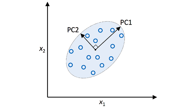
PCA is a linear transformation technique that identifies the directions that capture the most variation in the data and projects the data onto those directions, which are called principal components. Each principal component is a linear combination of the original variables, and the first principal component captures the most variation in the data, the second principal component captures the second-most variation, and so on. In the diagram below, there are two independent principal components PC1 and PC2. Note that PC1 represents the eigenvector which explains most of the information variance. PC2 represents lesser information (variance)

Explained variance is a statistical measure of how much variation in a dataset can be attributed to each of the principal components (eigenvectors) generated by the principal component analysis (PCA) method. In other words, it tells us how much of the total variance is “explained” by each component. This is important because it allows us to rank the components in order of importance, and to focus on the most important ones when interpreting the results of our analysis.
For example, let’s say you want to build a machine learning model to predict housing prices. The explained variance would tell us how much of the variation in housing prices can be explained by the model. In this case, a higher explained variance would be better because it would mean that the model is doing a better job of predicting housing prices.
The concept of Explained variance is useful in assessing how important each component is. In general, the larger the variance explained by a principal component, the more important that component is. Explained variance can be used to choose the number of dimensions to keep in a reduced dataset. It can also be used to assess the quality of the machine learning model. In general, a model with principal components having high explained variance will have good predictive power, while a model with principal components having low explained variance may not be as accurate.
# Example
Let’s understand the concept of Explained variance with examples. For example, if we have a dataset with 100 samples and 10 features, and we want to reduce it to two dimensions using PCA, we would expect the first component to explain about 86% of the variance (9/10), and the second component to explain about 14% (1/10). Explained variance can also be used to compare different PCA models. For example, if we compare two models that both reduce a dataset from 10 dimensions to 2, but one explains 80% of the variance and the other explains 95% of the variance, we would say that the latter model is better at representing the data.
# Formula
Explained variance can be represented as a function of ratio of related eigenvalue and sum of eigenvalues of all eigenvectors. Let’s say that there are N eigenvectors, then the explained variance for each eigenvector (principal component) can be expressed the ratio of eigenvalue of related eigenvalue $\lambda_i$ and sum of all eigenvalues $(\lambda_1 + \lambda_2 + … + \lambda_n)$ as the following:
$\frac{\lambda_i}{\lambda_1 + \lambda_2 + … +\lambda_n}$
Recall that a set of eigenvectors and related eigenvalues are found as part of eigen decomposition of transformation matrix which is covariance matrix in case of principal component analysis (PCA). These eigenvectors represent the principal components that contain most of the information (variance) represented using features (independent variables). The explained variance ratio represents the variance explained using a particular eigenvector.
How to determine Explained Variance using Python Code
The explained variance can be calculated using two techniques. Kaggla Data related to campus placement is used in the code given in the following sections.
- sklearn PCA class
- Custom Python code (without sklearn PCA) for determining explained variance
Sklearn PCA Class for determining Explained Variance
In this section, you will learn the code which makes use of PCA class of sklearn.decomposition for doing eigen decomposition of transformation matrix (Covariance matrix created using X_train_std in example given below). Here is the snapshot of the data after being cleaned up.

Note some of the following in the python code given below:
- explained_variance_ratio_ method of PCA is used to get the ration of variance (eigenvalue / total eigenvalues)
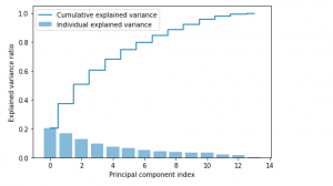
- Bar chart is used to represent individual explained variances.
- Step plot is used to represent the variance explained by different principal components.
- Data needs to be scaled before applying PCA technique.
#
# Scale the dataset; This is very important before you apply PCA
#
from sklearn.preprocessing import StandardScaler
sc = StandardScaler()
sc.fit(X_train)
X_train_std = sc.transform(X_train)
X_test_std = sc.transform(X_test)
#
# Instantiate PCA
#
pca = PCA()
#
# Determine transformed features
#
X_train_pca = pca.fit_transform(X_train_std)
#
# Determine explained variance using explained_variance_ration_ attribute
#
exp_var_pca = pca.explained_variance_ratio_
#
# Cumulative sum of eigenvalues; This will be used to create step plot
# for visualizing the variance explained by each principal component.
#
cum_sum_eigenvalues = np.cumsum(exp_var_pca)
#
# Create the visualization plot
#
plt.bar(range(0,len(exp_var_pca)), exp_var_pca, alpha=0.5, align='center', label='Individual explained variance')
plt.step(range(0,len(cum_sum_eigenvalues)), cum_sum_eigenvalues, where='mid',label='Cumulative explained variance')
plt.ylabel('Explained variance ratio')
plt.xlabel('Principal component index')
plt.legend(loc='best')
plt.tight_layout()
plt.show()
The Python code given above results in the following plot.

Custom Python Code (without using sklearn PCA) for determining Explained Variance
In this section, you will learn about how to determine explained variance without using sklearn PCA. Note some of the following in the code given below:
- Training data was scaled
- eigh method of numpy.linalg class is used.
- Covariance matrix of training dataset was created
- Eigenvalues and eigenvectors of covariance matrix was determined
- Explained variance was calculated
- Visualization plot was created for visualizing explained variance.
#
# Scale the dataset; This is very important before you apply PCA
#
from sklearn.preprocessing import StandardScaler
sc = StandardScaler()
sc.fit(X_train)
X_train_std = sc.transform(X_train)
X_test_std = sc.transform(X_test)
#
# Import eigh method for calculating eigenvalues and eigenvectirs
#
from numpy.linalg import eigh
#
# Determine covariance matrix
#
cov_matrix = np.cov(X_train_std, rowvar=False)
#
# Determine eigenvalues and eigenvectors
#
egnvalues, egnvectors = eigh(cov_matrix)
#
# Determine explained variance
#
total_egnvalues = sum(egnvalues)
var_exp = [(i/total_egnvalues) for i in sorted(egnvalues, reverse=True)]
#
# Plot the explained variance against cumulative explained variance
#
import matplotlib.pyplot as plt
cum_sum_exp = np.cumsum(var_exp)
plt.bar(range(0,len(var_exp)), var_exp, alpha=0.5, align='center', label='Individual explained variance')
plt.step(range(0,len(cum_sum_exp)), cum_sum_exp, where='mid',label='Cumulative explained variance')
plt.ylabel('Explained variance ratio')
plt.xlabel('Principal component index')
plt.legend(loc='best')
plt.tight_layout()
plt.show()
Here is how the explained variance plot would look like:

References
Conclusion
Here are the conclusions / learning from this post:
- Explained variance represents the information explained using different principal components (eigenvectors)
- Explained variance is calculated as ratio of eigenvalue of a articular principal component (eigenvector) with total eigenvalues.
- Explained variance can be calculated as the attribute explained_variance_ratio_ of PCA instance created using sklearn.decomposition PCA class.
- The Watermelon Effect: When Green Metrics Lie - January 25, 2026
- Coefficient of Variation in Regression Modelling: Example - November 9, 2025
- Chunking Strategies for RAG with Examples - November 2, 2025

I found it very helpful. However the differences are not too understandable for me