
In this post, you will learn about the concepts of negative binomial distribution explained using real-world examples and Python code. We will go over some of the following topics to understand negative binomial distribution:
- What is negative binomial distribution?
- What is difference between binomial and negative binomial distribution?
- Negative binomial distribution real-world examples
- Negative binomial distribution Python example
What is Negative Binomial Distribution?
Negative binomial distribution is a discrete probability distribution representing the probability of random variable, X, which is number of Bernoulli trials required to have r number of successes. This random variable is called as negative binomial random variable. And, the experiment representing X number of Bernoulli trials required to product r successes is called as negative binomial experiment. Let’s understand the concept with the example of tossing a coin. Let’s say we want to continue flipping the coin until 3 heads come. This experiment of flipping a coin until 3 heads (r=3) come can be called as negative binomial experiment. And, the number of times the coin need to be flipped in each experiment represent the value of negative binomial random variable, X.
The negative binomial experiment would have the following properties:
- The experiment consists of X repeated trials until r successes occur.
- Each trial could result in only two outcomes – success or failure. In other words, the trial must be Bernoulli trial
- The probability of success on each trial is same as P
- The trials are independent of each other. Thus, in tossing coin experiment, head in one trial will not impact what appears in the next trial. It could be either head or tail.
The negative binomial distribution can be represented as the following when X represents the number of trials needed to get r successes where the probability of success in each trial is P.
[latex]\Large B^{*}(X; r, P)[/latex]
.
The expected value / mean of the negative binomial distribution is defined as the expected / mean number of trials required to achieve r successes where the probability of success is P.
[latex]\Large \mu_{X} = \frac{r}{P}[/latex]
.
Alternative Definitions of Negative Binomial Distribution
Negative binomial distribution definitions vary with the definition of negative binomial random variable. Here are different definitions of the negative binomial random variable:
- Negative binomial random variable X represents number of successes before the binomial experiment results in k failures. The probability of success is P and failure is 1 – P.
[latex]\Large \mu_{X} = k*\frac{P}{(1-P)}[/latex]
.
- Negative binomial random variable X represents number of failures before the binomial experiment results in r successes. The probability of success is P and failure is 1 – P.
[latex]\Large \mu_{X} = r*\frac{1-P}{P}[/latex]
.
Difference between Binomial & Negative Binomial Distribution
To understand the difference between binomial and negative binomial distribution, lets understand the difference between binomial and negative binomial experiment.
Binomial experiment is getting number of successes in N number of Bernoulli trials. The binomial random variable is number of successes. In binomial distribution, the number of trials are fixed.
Negative binomial experiment is about performing Bernoulli trials until r successes is achieved. The negative binomial random variable, X, is number of trials which are required to achieve r successes. In negative binomial distribution, the number of trials are not fixed.
In both the above cases, the following properties holds good:
- The trials have only two outcomes – success and failures. In other words, the trials are Bernoulli trials.
- The trials are independent of each other. The outcome from one trial does not impact the following trials.
- The probability of getting success in each trial is one and the same.
Negative Binomial Distribution Real-world Examples
Here are some real-world examples of negative binomial distribution:
- Let’s say there is 10% chance of a sales person getting to schedule a follow-up meeting with the prospect in the phone call. The number of calls that the sales person would need to get 3 follow-up meetings would follow the negative binomial distribution. Thus, one will be able to calculate what is the probability that the sales person get 3 follow-up calls set in the 10th call. As per the alternative definitions, the number of rejections before which the sales person achieve 3 follow-up calls will follow the negative binomial distribution.
- Let’s say there is 30% chance that a basketball player will be able to get a perfect score in the free throw. The number of free throws that may be required to get the first score will follow the negative binomial distribution. Recall that this will also follow the geometric distribution. Geometric distribution, that way, is considered as the special case of negative binomial distribution. This example can also be read as the following – Number of free throw failures which will required to get the first perfect score will follow negative binomial distribution.
Negative Binomial Distribution Python Example
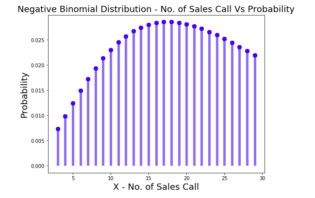
Here is the Python code representing negative binomial distribution. Pay attention that Scipy.stats nbinom can be used to calculate probability distribution.
import numpy as np
from scipy.stats import nbinom
import matplotlib.pyplot as plt
#
# X = Discrete negative binomial random variable representing number of sales call required to get r=3 leads
# P = Probability of successful sales call
#
X = np.arange(3, 30)
r = 3
P = 0.1
#
# Calculate geometric probability distribution
#
nbinom_pd = nbinom.pmf(X, r, P)
#
# Plot the probability distribution
#
fig, ax = plt.subplots(1, 1, figsize=(8, 6))
ax.plot(X, nbinom_pd, 'bo', ms=8, label='nbinom pmf')
ax.plot(X, nbinom_pd, 'bo', ms=8, label='nbinom pmf')
plt.ylabel("Probability", fontsize="18")
plt.xlabel("X - No. of Sales Call", fontsize="18")
plt.title("Negative Binomial Distribution - No. of Sales Call Vs Probability", fontsize="18")
ax.vlines(X, 0, nbinom_pd, colors='b', lw=5, alpha=0.5)
Here is how the negative binomial distribution plot would look like:
Conclusions
Here is the summary of what you learned in this post regarding negative binomial distribution:
- Negative binomial distribution is a discrete probability distribution which models the number of trials it will take to achieve r successes. Alternative definition is number of failures it would take to r successes.
- Negative binomial experiment is number of Bernoulli trials it will take to achieve r successes.
- Negative binomial random variable is number of Bernoulli trials to get r successes.

Check out my latest book titled as First Principles Thinking: Building winning products using first principles thinking.
- Mathematics Topics for Machine Learning Beginners - July 6, 2025
- Questions to Ask When Thinking Like a Product Leader - July 3, 2025
- Three Approaches to Creating AI Agents: Code Examples - June 27, 2025
I found it very helpful. However the differences are not too understandable for me