Ever wondered how insurance companies determine the premiums you pay for your health insurance? Predicting insurance premiums is more than just a numbers game—it’s a task that can impact millions of lives. In this blog, we’ll demystify this complex process by walking you through an end-to-end example of predicting health insurance premium charges by demonstrating with Python code example. Specifically, we’ll use a linear regression model to predict these charges based on various factors like age, BMI, and smoking status. Whether you’re a beginner in data science or a seasoned professional, this blog will offer valuable insights into building and evaluating regression models.
What is Linear Regression?
Linear Regression is a supervised machine learning algorithm used for predicting a numerical dependent variable based on one or more features (independent variables). In the case of insurance, the target variable is the insurance premium (charge), and the features could be age, gender, BMI, and so on. For learning more about linear regression models, check out my other related blogs:
The following are key steps which will be explained while building the regression models for predicting health insurance premium charges:
- Exploratory data analysis
- Feature engineering
- Data preparation
- Building the model
- Model evaluation
Exploratory Data Analysis (EDA) of Insurance Data
We will work with the insurance data which can be found on this Github page – Insurance Linear Regression Model Example. The dataset contains the following columns:
- age: Age of the insured
- sex: Gender of the insured
- bmi: Body Mass Index
- children: Number of dependents/children
- smoker: Smoking status
- region: Geographical region
- charges: Insurance premium charges
First and foremost, we will load the data.
import pandas as pd

# Load the data
file_path = '/path/to/insurance.csv'
insurance_data = pd.read_csv(file_path)

# Display the first few rows
print(insurance_data.head())
Exploratory Data Analysis (EDA) is an essential step to understand the data before building any machine learning model. We’ll look into the following commonly explored aspects:
- Descriptive Statistics
- Data Types and Missing Values
- Univariate Analysis (Distribution of individual features)
- Bivariate Analysis (Correlation between features and target variable)
Descriptive statistics
Let’s start with the descriptive statistics to get an overview of the numerical columns in the dataset.
# Generate descriptive statistics of the numerical columns
insurance_data.describe()
The descriptive statistics for the numerical columns are as follows:
- Age: Ranges from 18 to 64 years, with a mean age of approximately 39.2 years.
- BMI: Ranges from 15.96 to 53.13, with a mean BMI of around 30.7.
- Children: Ranges from 0 to 5, with an average of approximately 1.1 children.
- Charges: The insurance premium charges vary significantly, ranging from 1121.87 to 63770.43, with a mean of approximately 13270.42.
Data types & missing values
Next, let’s check the data types of each column and see if there are any missing values.
# Check data types and missing values
data_info = pd.DataFrame({
    'Data Type': insurance_data.dtypes,
    'Missing Values': insurance_data.isnull().sum(),
    'Unique Values': insurance_data.nunique()
})

data_info
The data types and missing values are as follows:
- Age: Integer type, no missing values
- Sex: Object (categorical), no missing values
- BMI: Float, no missing values
- Children: Integer type, no missing values
- Smoker: Object (categorical), no missing values
- Region: Object (categorical), no missing values
- Charges: Float, no missing values
All columns have appropriate data types and there are no missing values, which is a great news. Handling missing values is a critical step in the data preprocessing pipeline, as most machine learning algorithms cannot work with missing data directly. Here are some common techniques to deal with missing values:
- Removing rows and / or columns
- Data imputation (mean/median/mode)
- Advanced data imputation (regression modeling)
Univariate analysis
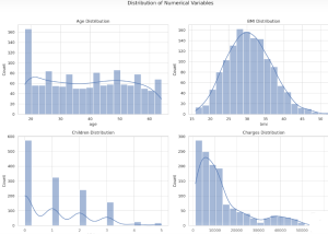
Let’s move on to the univariate analysis. We’ll start by visualizing the distribution of the numerical variables (age, bmi, children, and charges) and then take a look at the categorical variables (sex, smoker, and region).
We’ll plot histograms for age, bmi, children and charges to understand their distributions.
import matplotlib.pyplot as plt
import seaborn as sns

# Set the style for the visualizations
sns.set(style="whitegrid")

# Plot histograms for numerical variables
fig, axes = plt.subplots(2, 2, figsize=(14, 10))
fig.suptitle('Distribution of Numerical Variables')

sns.histplot(insurance_data['age'], kde=True, bins=20, ax=axes[0, 0])
axes[0, 0].set_title('Age Distribution')

sns.histplot(insurance_data['bmi'], kde=True, bins=20, ax=axes[0, 1])
axes[0, 1].set_title('BMI Distribution')

sns.histplot(insurance_data['children'], kde=True, bins=20, ax=axes[1, 0])
axes[1, 0].set_title('Children Distribution')

sns.histplot(insurance_data['charges'], kde=True, bins=20, ax=axes[1, 1])
axes[1, 1].set_title('Charges Distribution')

plt.tight_layout(rect=[0, 0, 1, 0.96])
plt.show()
Here’s what we can observe from the histograms:
- Age Distribution: Most of the insured individuals are between 20 and 30 years old, with fewer individuals above 50.
- BMI Distribution: The BMI appears to be normally distributed, centering around 30.
- Children Distribution: A large number of insured individuals have no children, followed by those with 1 or 2 children.
- Charges Distribution: The distribution of charges is right-skewed, indicating that most people pay lower premiums, but there are some who pay significantly higher premiums.
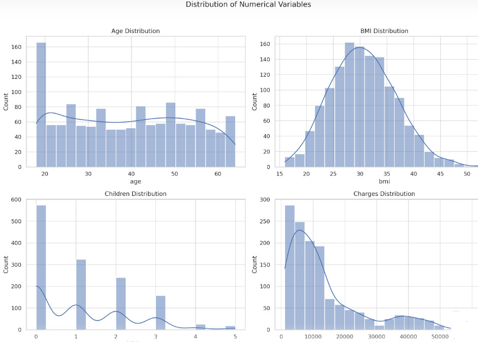
Next, let’s look at the distribution of the categorical variables (sex, smoker, and region) using bar plots.
# Plot bar plots for categorical variables
fig, axes = plt.subplots(1, 3, figsize=(18, 6))
fig.suptitle('Distribution of Categorical Variables')

sns.countplot(x='sex', data=insurance_data, ax=axes[0])
axes[0].set_title('Gender Distribution')

sns.countplot(x='smoker', data=insurance_data, ax=axes[1])
axes[1].set_title('Smoker Distribution')

sns.countplot(x='region', data=insurance_data, ax=axes[2])
axes[2].set_title('Region Distribution')

plt.tight_layout(rect=[0, 0, 1, 0.96])
plt.show()
The bar plots for the categorical variables show the following:
- Gender Distribution: The dataset is fairly balanced between males and females.
- Smoker Distribution: The number of non-smokers is significantly higher than that of smokers.
- Region Distribution: The data is relatively evenly distributed across the four regions, with the ‘southeast’ region having a slightly higher representation.
Now that we have a better understanding of the individual features, let’s move on to bivariate analysis to explore the relationships between these features and the target variable (charges).
Bivariate Analysis
In the bivariate analysis, we’ll focus on understanding the relationship between the individual features and the target variable, charges.
We’ll start by plotting scatter plots between the numerical variables (age, bmi, children) and charges to observe any trends or patterns.
# Plot scatter plots for numerical variables vs charges
fig, axes = plt.subplots(1, 3, figsize=(18, 6))
fig.suptitle('Scatter Plots of Numerical Variables vs Charges')

sns.scatterplot(x='age', y='charges', data=insurance_data, ax=axes[0])
axes[0].set_title('Age vs Charges')

sns.scatterplot(x='bmi', y='charges', data=insurance_data, ax=axes[1])
axes[1].set_title('BMI vs Charges')

sns.scatterplot(x='children', y='charges', data=insurance_data, ax=axes[2])
axes[2].set_title('Children vs Charges')

plt.tight_layout(rect=[0, 0, 1, 0.96])
plt.show()
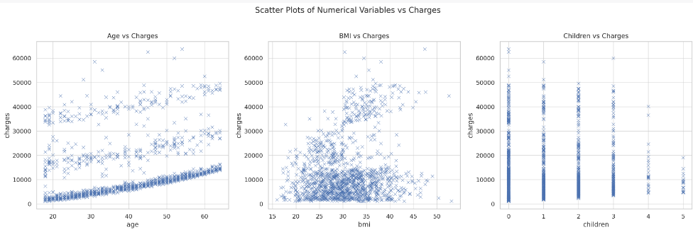
Here are some observations from the scatter plots:
- Age vs Charges: There seems to be a positive correlation between age and insurance charges, indicating that older individuals are likely to be charged higher premiums.
- BMI vs Charges: There is a general trend showing higher charges for individuals with higher BMI, although the relationship is not as clear-cut.
- Children vs Charges: The relationship between the number of children and charges is not very clear from the scatter plot. Charges appear to be distributed across the range for different numbers of children.
Next, let’s look at how the categorical variables (sex, smoker and region) relate to the insurance charges. We’ll use box plots for this analysis.
# Plot box plots for categorical variables vs charges
fig, axes = plt.subplots(1, 3, figsize=(18, 6))
fig.suptitle('Box Plots of Categorical Variables vs Charges')

sns.boxplot(x='sex', y='charges', data=insurance_data, ax=axes[0])
axes[0].set_title('Gender vs Charges')

sns.boxplot(x='smoker', y='charges', data=insurance_data, ax=axes[1])
axes[1].set_title('Smoker vs Charges')

sns.boxplot(x='region', y='charges', data=insurance_data, ax=axes[2])
axes[2].set_title('Region vs Charges')

plt.tight_layout(rect=[0, 0, 1, 0.96])
plt.show()
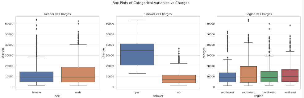
The box plots reveal the following insights:
- Gender vs Charges: The median insurance charges are quite similar for both genders, although males seem to have a slightly higher range of charges.
- Smoker vs Charges: There’s a significant difference in charges between smokers and non-smokers, with smokers generally facing much higher premiums.
- Region vs Charges: The charges appear to be distributed fairly similarly across different regions, with no substantial differences.
The EDA has provided valuable insights into how various features relate to insurance charges. Now we are better equipped to build a linear regression model for predicting insurance premiums. As a next step, we will prepare data before we train the model.
Feature Engineering for Building Linear Regression Model
Before building the model, let’s summarize our understanding of the features based on the exploratory data analysis:
- Age: Positively correlated with charges; older individuals tend to have higher charges.
- BMI: Generally, higher BMI corresponds to higher charges, though the relationship isn’t perfectly linear.
- Children: The number of children doesn’t show a clear trend but could still provide some predictive power.
- Sex: Gender doesn’t show a significant difference in charges, but we’ll include it for a more comprehensive model.
- Smoker: A very strong predictor; smokers have much higher charges.
- Region: Charges are distributed fairly evenly across regions, but we’ll include it to capture any regional nuances.
Based on the above, the following is the rationale for feature selection:
- Include: Age, BMI, Children, Smoker — these have shown correlations or differences in charges during the EDA.
- Conditional Include: Sex, Region — these don’t show strong correlations but could improve the model’s performance by capturing underlying patterns.
Data Preparation for Building Linear Regression Model
The next step is data preparation for modeling, which includes encoding categorical variables and splitting the data into training and test sets.
- Numerical features (age, bmi, children) have been standardized, meaning they’ve been scaled to have a mean of 0 and a standard deviation of 1. sklearn.preprocessing.StandardScaler is used for standardizing numerical data.
- Categorical features (sex, smoker, region) have been one-hot encoded to convert them into a format that can be provided to machine learning algorithms. sklearn.preprocessing.OneHotEncoder is used for encoding categorical variables.
In addition, we also split the data in training and testing set. This would be used for training the model and evaluating the model performance.
from sklearn.model_selection import train_test_split
from sklearn.preprocessing import StandardScaler, OneHotEncoder
from sklearn.compose import ColumnTransformer

# Define the features and the target
X = insurance_data.drop('charges', axis=1)
y = insurance_data['charges']

# Identify numerical and categorical columns
numerical_cols = ['age', 'bmi', 'children']
categorical_cols = ['sex', 'smoker', 'region']

# Preprocessing for numerical data: standardization
numerical_transformer = StandardScaler()

# Preprocessing for categorical data: one-hot encoding
categorical_transformer = OneHotEncoder(handle_unknown='ignore')

# Bundle preprocessing for numerical and categorical data
preprocessor = ColumnTransformer(
    transformers=[
        ('num', numerical_transformer, numerical_cols),
        ('cat', categorical_transformer, categorical_cols)])

# Split data into train and test sets
X_train, X_test, y_train, y_test = train_test_split(X, y, test_size=0.2, random_state=0)
Train the Linear Regression Model for Predicting Insurance Premium Charges
The next step is training the linear regression model to predict the health insurance premium charges.
from sklearn.pipeline import Pipeline
from sklearn.linear_model import LinearRegression

# Define the model
model = LinearRegression()

# Create and evaluate the pipeline
pipeline = Pipeline(steps=[('preprocessor', preprocessor),
                           ('model', model)
                          ])

# Fit the model using training data
pipeline.fit(X_train, y_train)
Evaluating the Linear Regression Model
Now that the model is trained, its time to evaluate the linear regression model performance. Here is the code:
from sklearn.metrics import mean_squared_error, mean_absolute_error, r2_score

# Predict on test data
y_pred = pipeline.predict(X_test)

# Evaluate the model
mse = mean_squared_error(y_test, y_pred)
rmse = mean_squared_error(y_test, y_pred, squared=False)
mae = mean_absolute_error(y_test, y_pred)
r2 = r2_score(y_test, y_pred)

evaluation_metrics = {
    'Mean Squared Error': mse,
    'Root Mean Squared Error': rmse,
    'Mean Absolute Error': mae,
    'R-squared': r2
}

evaluation_metrics
The regression model’s performance metrics on the test set are as follows:
- Mean Squared Error (MSE): 31,860,50031,860,500
- Root Mean Squared Error (RMSE): 5,644.515,644.51
- Mean Absolute Error (MAE): 3,942.913,942.91
- R-squared: 0.8000.800
The following can be interpreted based on above metrics:
- The R-squared value of 0.8000.800 suggests that the model explains approximately 80% of the variance in the insurance charges, which is quite good.
- RMSE and MAE give us an idea of the average prediction error in the units of the target variable (charges). Lower values for these metrics are generally better.
Conclusion
So, there we have it—a comprehensive guide to predicting insurance premiums using Linear Regression. From understanding the intricacies of insurance data to diving deep into exploratory data analysis, and finally building and evaluating our model, we’ve covered quite a bit of ground. But what did we really learn?
- Linear Regression is Powerful Yet Simple: Even with its simplicity, a Linear Regression model can offer a high degree of accuracy for predicting insurance premiums. It’s a great starting point for anyone new to machine learning.
- Data Understanding is Crucial: Before jumping into any machine learning model, a thorough exploratory data analysis (EDA) is indispensable. It not only helps in feature selection but also gives you a better understanding of the data you’re working with.
- Preprocessing Matters: Handling missing values, encoding categorical variables, and standardizing features are critical steps that can significantly impact your model’s performance.
- Evaluation is Key: Always use metrics like MSE, RMSE, MAE, and R-squared to evaluate your model’s performance. It’s not just about building a model; it’s about understanding how well it’s performing.

Check out my latest book titled as First Principles Thinking: Building winning products using first principles thinking.
- Mathematics Topics for Machine Learning Beginners - July 6, 2025
- Questions to Ask When Thinking Like a Product Leader - July 3, 2025
- Three Approaches to Creating AI Agents: Code Examples - June 27, 2025
I found it very helpful. However the differences are not too understandable for me