Hidden Markov models (HMMs) are a type of statistical modeling that has been used for several years. They have been applied in different fields such as medicine, computer science, and data science. The Hidden Markov model (HMM) is the foundation of many modern-day data science algorithms. It has been used in data science to make efficient use of observations for successful predictions or decision-making processes. This blog post will cover hidden Markov models with real-world examples and important concepts related to hidden Markov models.
What are Markov Models?
Markov models are named after Andrey Markov, who first developed them in the early 1900s. Markov models are a type of probabilistic model that is used to predict the future state of a system, based on its current state. In other words, Markov models are used to predict the future state based on the current hidden or observed states. Markov model is a finite-state machine where each state has an associated probability of being in any other state after one step. They can be used to model real-world problems where hidden and observable states are involved. Markov models can be classified into hidden and observable based on the type of information available to use for making predictions or decisions. Hidden Markov models deal with hidden variables that cannot be directly observed but only inferred from other observations, whereas in an observable model also termed as Markov chain, hidden variables are not involved.
To better understand Markov models, let’s look at an example. Say you have a bag of marbles that contains four marbles: two red marbles and two blue marbles. You randomly select a marble from the bag, note its color, and then put it back in the bag. After repeating this process several times, you begin to notice a pattern: The probability of selecting a red marble is always two out of four, or 50%. This is because the probability of selecting a particular color of marble is determined by the number of that color of marble in the bag. In other words, the past history (i.e., the contents of the bag) determines the future state (i.e., the probability of selecting a particular color of marble).
This example illustrates the concept of a Markov model: the future state of a system is determined by its current state and past history. In the case of the bag of marbles, the current state is determined by the number of each color of marble in the bag. The past history is represented by the contents of the bag, which determine the probabilities of selecting each color of marble.
Markov models have many applications in the real world, including predicting the weather, stock market prices, and the spread of disease. Markov models are also used in natural language processing applications such as speech recognition and machine translation. In speech recognition, Markov models are used to identify the correct word or phrase based on the context of the sentence. In machine translation, Markov models are used to select the best translation for a sentence based on the translation choices made for previous sentences in the text.
What is Markov Chain?
Markov chains, named after Andrey Markov, can be thought of as a machine or a system that hops from one state to another, typically forming a chain. Markov chains have the Markov property, which states that the probability of moving to any particular state next depends only on the current state and not on the previous states.
A Markov chain consists of three important components:
- Initial probability distribution: An initial probability distribution over states, πi is the probability that the Markov chain will start in a certain state i. Some states j may have πj = 0, meaning that they cannot be initial states
- One or more states
- Transition probability distribution: A transition probability matrix A where each [latex]a_{ij}[/latex] represents the probability of moving from state I to state j
The diagram below represents a Markov chain where there are three states representing the weather of the day (cloudy, rainy, and sunny). And, there are transition probabilities representing the weather of the next day given the weather of the current day.
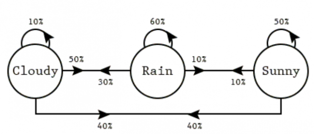
There are three different states such as cloudy, rain, and sunny. The following represent the transition probabilities based on the above diagram:
- If sunny today, then tomorrow:
- 50% probability for sunny
- 10% probability for rainy
- 40% probability for cloudy
- If rainy today, then tomorrow:
- 10% probability for sunny
- 60% probability for rainy
- 30% probability for cloudy
- If cloudy today, then tomorrow:
- 40% probability for sunny
- 50% probability for rainy
- 10% probability for cloudy
Using this Markov chain, what is the probability that the Wednesday will be cloudy if today is sunny. The following are different transitions that can result in a cloudy Wednesday given today (Monday) is sunny.
- Sunny – Sunny (Tuesday) – Cloudy (Wednesday): The probability to a cloudy Wednesday can be calculated as 0.5 x 0.4 = 0.2
- Sunny – Rainy (Tuesday) – Cloudy (Wednesday): The probability of a cloudy Wednesday can be calculated as 0.1 x 0.3 = 0.03
- Sunny – Cloudy (Tuesday) – Cloudy (Wednesday): The probability of a cloudy Wednesday can be calculated as 0.4 x 0.1 = 0.04
The total probability of a cloudy Wednesday = 0.2 + 0.03 + 0.04 = 0.27.
As shown above, the Markov chain is a process with a known finite number of states in which the probability of being in a particular state is determined only by the previous state.
What are Hidden Markov models (HMM)?
The hidden Markov model (HMM) is another type of Markov model where there are few states which are hidden. This is where HMM differs from a Markov chain. HMM is a statistical model in which the system being modeled are Markov processes with unobserved or hidden states. It is a hidden variable model which can give an observation of another hidden state with the help of the Markov assumption. The hidden state is the term given to the next possible variable which cannot be directly observed but can be inferred by observing one or more states according to Markov’s assumption. Markov assumption is the assumption that a hidden variable is dependent only on the previous hidden state. Mathematically, the probability of being in a state at a time t depends only on the state at the time (t-1). It is termed a limited horizon assumption. Another Markov assumption states that the conditional distribution over the next state, given the current state, doesn’t change over time. This is also termed a stationary process assumption.
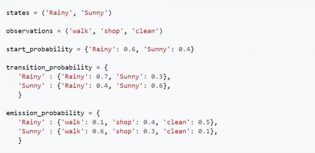
A Markov model is made up of two components: the state transition and hidden random variables that are conditioned on each other. However, A hidden Markov model consists of five important components:
- Initial probability distribution: An initial probability distribution over states, πi is the probability that the Markov chain will start in state i. Some states j may have πj = 0, meaning that they cannot be initial states. The initialization distribution defines each hidden variable in its initial condition at time t=0 (the initial hidden state).
- One or more hidden states
- Transition probability distribution: A transition probability matrix where each [latex]a_{ij}[/latex] represents the probability of moving from state i to state j. The transition matrix is used to show the hidden state to hidden state transition probabilities.
- A sequence of observations
- Emission probabilities: A sequence of observation likelihoods, also called emission probabilities, each expressing the probability of an observation [latex]o_{i}[/latex] being generated from a state I. The emission probability is used to define the hidden variable in terms of its next hidden state. It represents the conditional distribution over an observable output for each hidden state at time t=0.
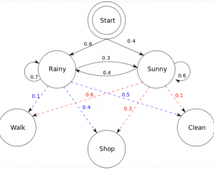
Let’s understand the above using the hidden Markov model representation shown below:
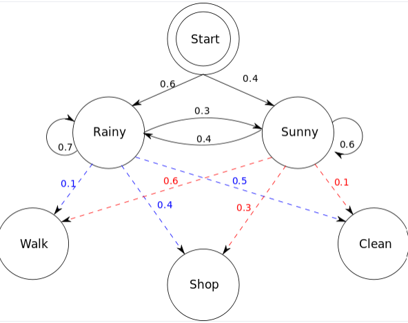
The hidden Markov model in the above diagram represents the process of predicting whether someone will be found to be walking, shopping, or cleaning on a particular day depending upon whether the day is rainy or sunny. The following represents five components of the hidden Markov model in the above diagram:
Let’s notice some of the following in the above picture:
- There are two hidden states such as rainy and sunny. These states are hidden because what is observed as the process output is whether the person is shopping, walking, or cleaning.
- The sequence of observations is shop, walk, and clean.
- An initial probability distribution is represented by start probability
- Transition probability represents the transition of one state (rainy or sunny) to another state given the current state
- Emission probability represents the probability of observing the output, shop, clean and walk given the states, rainy or sunny.
The Hidden Markov model is a special type of Bayesian network that has hidden variables which are discrete random variables. The first-order hidden Markov model allows hidden variables to have only one state and the second-order hidden Markov models allow hidden states to be having two or more two hidden states.
The hidden Markov model represents two different states of variables: Hidden state and observable state. A hidden state is one that cannot be directly observed or seen. An observable state is one that can be observed or seen. One hidden state can be associated with many observable states and one observable state may have more than hidden states. The hidden Markov model uses the concept of probability to identify whether there will be an emission from the hidden state to another hidden state or from hidden states to observable states.
Real-world examples of Hidden Markov Models (HMM)
Here are a few real-world examples where the hidden Markov models are used:
- Retail scenario: Now if you go to the grocery store once per week, it is relatively easy for a computer program to predict exactly when your shopping trip will take more time. The hidden Markov model calculates which day of visiting takes longer compared with other days and then uses that information in order to determine why some visits are taking long while others do not seem too problematic for shoppers like yourself. Another example from e-commerce where hidden Markov models are used is the recommendation engine. The hidden Markov models try to predict the next item that you would like to buy.
- Travel scenario: By using hidden Markov models, airlines can predict how long it will take a person to finish checking out from an airport. This allows them to know when they should start boarding passengers!
- Medical Scenario: The hidden Markov models are used in various medical applications, where it tries to find out the hidden states of a human body system or organ. For example, cancer detection can be done by analyzing certain sequences and determining how dangerous they might pose for the patient. Another example where hidden Markov models get used is for evaluating biological data such as RNA-Seq, ChIP-Seq, etc., that help researchers understand gene regulation. Using the hidden Markov model, doctors can predict the life expectancy of people based on their age, weight, height, and body type.
- Marketing scenario: As marketers utilize a hidden Markov model, they can understand at what stage of their marketing funnel users are dropping off and how to improve user conversion rates.
What are some libraries which can be used for training hidden Markov models?
- One of the popular hidden Markov model libraries is PyTorch-HMM, which can also be used to train hidden Markov models. The library is written in Python and it can be installed using PIP.
- HMMlearn: Hidden Markov models in Python
- PyHMM: PyHMM is a hidden Markov model library for Python.
- DeepHMM: A PyTorch implementation of a Deep Hidden Markov Model
- HiddenMarkovModels.jl
- HMMBase.jl
Great Tutorials on Hidden Markov Models
Here are some great tutorials I could find on Youtube. Pls feel free to suggest any other tutorials you have come across.
Conclusion
In conclusion, this blog has explored what a Markov Model is, what Hidden Markov Models are, and some of their real-world applications. It is important to have an understanding of these topics if one wants to use them in a data science project. With the increasing complexity of datasets, the use of these models can provide invaluable insights into data correlations and trends.

Check out my latest book titled as First Principles Thinking: Building winning products using first principles thinking.
- Mathematics Topics for Machine Learning Beginners - July 6, 2025
- Questions to Ask When Thinking Like a Product Leader - July 3, 2025
- Three Approaches to Creating AI Agents: Code Examples - June 27, 2025
Loved this Ajitesh! Really interesting and concise stuff. Thanks for uploading this!
Thank you for making it so easy to understand!
Dear sir, I’m a PhD students in Nigeria. I’m working on face recognition and extraction. I s there a way I can use HMM in my research. I’m new to HMM but read several articles before coming across your article recently. I need help. Thank you sir
My God!
What would be ur hidden variables n observed variables in this instance ?
Use deep learning..convolutional neural netwks for face recogn ition…it’s easier n much more straight forward.
Read prof bharatendra Rai tutorials in YouTube on the same.
clear, to the point explanation with examples.
Thanks very much.
You makes my day bright
I need help but I don’t know whom to contact. I would like to use HMM for dynamic gesture detection. I am trying to use it in a way that I would capture the movement of object and detect it using HMM .