Have you ever wondered how machine learning models transform their intricate calculations into clear, human-readable language? Or how your smartphone knows exactly what you’re going to type next before you even start typing? These everyday marvels are powered by a critical component of natural language processing (NLP) known as ‘decoding methods‘. But how do these methods work, and why are there different types?
In the vast field of machine learning, a primary challenge in natural language processing tasks is converting a model’s computational output into an understandable and coherent text. Whether it’s autocompleting your sentences, translating text from one language to another, or generating a news article, these tasks involve a complex process called ‘sequence generation’. However, sequence generation isn’t as simple as picking words out of thin air. Given the extensive vocabulary and virtually infinite combinations of words and phrases, choosing the ‘right’ sequence of words can be a herculean task. How can we effectively navigate this enormous space of possibilities? How can we ensure that the generated text is not only grammatically correct but also makes sense and maintains context?
Enter decoding methods. They help in transforming the model’s raw, probabilistic output into coherent sequences of text. Among the various decoding methods, two commonly used strategies are Greedy Search and Beam Search. In this blog, we will delve deep into the world of Greedy Search and Beam Search decoding methods. We will explain these key concepts, illustrate them with real-world examples, and shed light on how these powerful techniques enable our machines to ‘speak’ and ‘write’.
What’s Decoding Method in NLP?
In the context of natural language processing and language models, “decoding” refers to the process of transforming the model’s output into a human-understandable format, typically a sequence of words or tokens.
Language models like GPT-2 or GPT-3 generate output in the form of a probability distribution over the entire vocabulary for each step in the sequence. This means that for a given input, the model will produce a list of probabilities, one for each word in its vocabulary, indicating how likely that word is to be the next word in the sequence.
However, this raw output isn’t directly useful. What we want is a sequence of words. Therefore, we need a method to “decode” this probability distribution into a sequence of words.
Why do we use the word “decoding”? It’s an analogy drawn from the concept of code and decoding in communication theory. In that context, a message is encoded into a format suitable for transmission, then decoded by the receiver back into the original message. Similarly, a language model encodes its understanding of the text in the form of probability distributions, and we must decode this output to generate human-readable text.
What is Greedy Search Decoding?
Greedy search is the simplest decoding method. At each step, it selects the word (token) with the highest probability and adds it to the sequence. This process continues until a stop condition is met, such as reaching an end token or a maximum sequence length.
Imagine you’re at a fruit market with a friend who has a quirky method for choosing fruits. Every time they choose, they pick the fruit they like most at that very moment without thinking about what they’ll want next. This method might not result in a varied fruit basket, but it’s quick and straightforward.
Now, let’s equate this to how a language model, using Greedy Search, might complete a sentence.
Given the sentence start: “My favorite fruit is ___.”
The model will predict the next word based on its training data. At each step, it picks the word with the highest probability without considering the broader context of the sentence.
1st Step: After “My”, the model might have high probabilities for “favorite”, “mother”, “dog”, etc. Since we’re using Greedy Search, it picks “favorite” as it has the highest probability.
2nd Step: For “My favorite”, the next word might be “fruit”, “color”, “thing”, etc. Again, it chooses the word with the highest probability, which is “fruit”.
3rd Step: Now, for “My favorite fruit”, the options might be “is”, “are”, “was”, etc. It selects “is”, having the highest probability.
4th Step: After “My favorite fruit is”, the options could be “apple”, “banana”, “grapes”, and so forth. If “apple” has the highest probability, it chooses that.
So, with Greedy Search, the completed sentence might be: “My favorite fruit is apple.”
Using Greedy Search is like how our friend at the fruit market selects fruits – always going for the most appealing option at the present moment without thinking ahead. While this method is simple and fast, it doesn’t always provide the best or most varied outcomes. In our sentence example, Greedy Search didn’t consider other possible, and maybe more interesting, continuations like “My favorite fruit is the exotic dragon fruit” because it was only focused on the highest immediate probability at each step.
The benefit of greedy search is its simplicity and computational efficiency. Because it only keeps track of the single most probable sequence, it requires less memory and computation compared to more complex decoding methods.
Drawbacks of Greedy Search Decoding Method
Greedy search has several key drawbacks, which primarily stem from its locally optimal decision-making strategy.
- Short-sightedness: Greedy search only looks for the best immediate option at each step and doesn’t consider the long-term implications of its choices. It’s akin to hiking in a mountain range and always choosing the immediate hilltop without considering the overall route to the highest peak. For example, suppose a language model is generating a story and has to choose between “The prince journeyed to the enchanted forest to find a…” and “The prince journeyed to the normal forest to find a…” At the particular decision point, ‘normal’ might be more likely than ‘enchanted’ in the model’s training data. However, ‘enchanted’ might lead to a more engaging and coherent story overall. Greedy search would miss out on the potentially better sequence because it only focuses on immediate gains.
- Lack of diversity: Greedy search tends to generate safe, repetitive, and often bland outputs. Because it always selects the most probable word at each step, it often defaults to common phrases and avoids less common but potentially more interesting choices. For example, if a model trained primarily on news articles might excessively generate phrases like “according to reports” or “experts say” since these phrases are very common in news writing.
- Propagation of errors: Once greedy search makes a sub-optimal decision, all future decisions are affected, and there’s no mechanism to correct the course. This problem is particularly acute in tasks like machine translation. For example, if the model mistranslates an early word in a sentence, that error could change the context for all subsequent words, leading to an entirely incorrect translation.
What is Beam Search Decoding?
Beam search is a more sophisticated decoding method that keeps track of multiple potential sequences at each step (the ‘beam width’). At each step, it generates multiple new sequences by appending every possible next word to each of the sequences it’s currently considering. It then selects the top ‘k’ most probable sequences from these new sequences, where ‘k’ is the beam width. Let’s try and understand with the help of a real-life example.
Imagine you’re trying to predict the next word in the sentence: “I like to eat ___.” Now, you could have many potential words to fill in the blank like “cake”, “apples”, “pasta”, etc. Let’s dive into Beam Search and see how it tackles this.
Beam Search in Action:
Let’s say our beam width �k is 2. This means that at each step, Beam Search will consider the top 2 sequences (combinations of words) based on their probabilities.
1st Step: The model predicts the probabilities for the next word after “I”. Let’s say the highest probabilities are for “like” and “am”. So, Beam Search keeps these two sequences:
- “I like”
- “I am”
2nd Step: Now, for each of the sequences, the model predicts the next word:
- For “I like”, it might predict “to” and “eating”.
- For “I am”, it might predict “happy” and “eating”.
This gives us the sequences:
- “I like to”
- “I like eating”
- “I am happy”
- “I am eating”
From these, it picks the top 2 sequences based on their probabilities. Let’s say it chooses:
- “I like to”
- “I am happy”
3rd Step: Repeat the process. For “I like to”, it predicts “eat” and “play”. For “I am happy”, it predicts “to” and “because”.
New sequences:
- “I like to eat”
- “I like to play”
- “I am happy to”
- “I am happy because”
From these, the top 2 sequences might be:
- “I like to eat”
- “I am happy because”
And this process continues until an end-of-sequence token is encountered or until a set sequence length is reached.
In contrast to Greedy Search which would have just taken the top prediction at each step (say, “I like to eat”), Beam Search considers multiple sequences. This makes it more flexible and increases the chances of it finding a better overall sequence. If Greedy Search had mistakenly chosen a less probable word in the first step, it might have ended up with a less coherent sentence in the end. But with Beam Search, by considering multiple sequences, there’s a higher likelihood of getting a more meaningful result.
The benefit of beam search is that it can explore a broader space of sequences and often generates more coherent and contextually appropriate sequences than greedy search. By keeping track of several promising sequences, it can avoid getting ‘stuck’ in less probable sequences because of locally optimal choices.
However, beam search requires more computational resources than greedy search, as it needs to maintain and calculate probabilities for ‘k’ sequences at each step. It also doesn’t guarantee to find the most probable sequence, especially if the beam width ‘k’ is too small compared to the size of the vocabulary.
Difference: Greedy Search & Beam Search Decoding Method
The following is a comparison of Greedy Search and Beam Search decoding method:
| Criteria | Greedy Search | Beam Search |
|---|---|---|
| Definition | A decoding method that always picks the next word (token) with the highest immediate probability. | A decoding method that keeps track of multiple potential sequences (beam width) selecting the top ‘k’ sequences at each step based on cumulative probabilities. |
| When to use | When computational efficiency is prioritized, and you need a quick, decent solution. | When a balance between computational cost and quality of output is required. Especially beneficial when higher quality or varied output is desired. |
| Example | Given the sentence “The cat is on the ___”, Greedy Search might complete it as “The cat is on the mat.” because “mat” has the highest immediate probability after “the”. | For the same sentence “The cat is on the ___”, Beam Search with a beam width of 2 might consider “mat” and “roof”. It might end up with “The cat is on the roof.” if this sequence has a higher overall probability, even if “roof” wasn’t the top single prediction initially. |
| Flexibility | Relatively rigid as it always selects the word with the highest immediate probability. | More flexible since it keeps multiple sequences in consideration, leading to a better exploration of possible outputs. |
| Risk of Local Minima | High. Can often get stuck in local optima because it doesn’t consider multiple possible sequences. | Reduced. The ability to track multiple sequences helps in navigating away from local optima and potentially finding a better overall output. |
| Computational Cost | Low. Since it only computes the next best token at each step, it’s computationally less expensive. | Higher than greedy search, as it needs to calculate probabilities for multiple sequences at each step. |
| Quality of Output | Can be suboptimal, especially in cases where looking ahead is crucial for a better sequence. | Generally produces better and more diverse results than greedy search, especially when the beam width is appropriately set. |
| Memory Requirement | Minimal. Only needs to remember the current sequence. | Higher. Has to remember multiple sequences (beam width) at each step. |
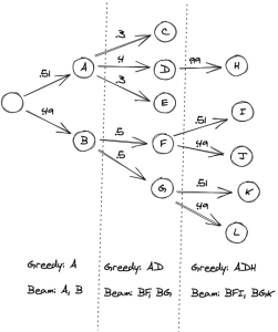
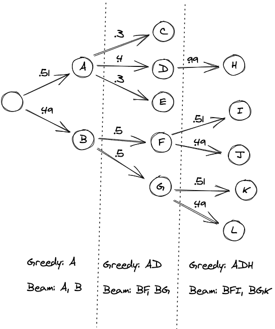
The picture below represents the difference in a visual manner.
Conclusion
Navigating the intricate realms of Natural Language Processing often lands us in front of pivotal choices. The decision between using Greedy Search and Beam Search decoding is one such crossroad. While Greedy Search offers a swift and computationally efficient approach, it may not always guarantee the most optimal or diverse results. Beam Search, on the other hand, brings a balanced blend of computational complexity and output quality, making it a popular choice for many NLP practitioners.
It’s essential to understand that there’s no one-size-fits-all. The best method often depends on the specific requirements of your task, computational resources, and desired output quality. Hopefully, with the insights from this blog, you’ll be better equipped to make an informed choice.

Check out my latest book titled as First Principles Thinking: Building winning products using first principles thinking.
- Mathematics Topics for Machine Learning Beginners - July 6, 2025
- Questions to Ask When Thinking Like a Product Leader - July 3, 2025
- Three Approaches to Creating AI Agents: Code Examples - June 27, 2025
I found it very helpful. However the differences are not too understandable for me