Last updated: 4th Dec, 2023.
In the fast-paced world of computer vision and image processing, the problem of image classification consistently stands out: the ability to effectively recognize and classify images. As we continue to digitize and automate our world, the demand for systems that can understand and interpret visual data is growing at an unprecedented rate. The challenge is not just about recognizing images – it’s about doing so accurately and efficiently. Traditional machine learning methods often fall short, struggling to handle the complexity and high dimensionality of image data. This is where Convolutional Neural Networks (CNNs) comes to rescue. And, there are different types of CNN architectures based on which a CNN model can be trained for image classification.

The CNN architecture is the most popular deep learning framework. CNNs shown remarkable success in tackling the problem of image recognition, bringing a newfound level of precision and scalability. But not all CNNs are created equal, and understanding the different types of CNN architectures is key to leveraging their full potential. In this blog post, we will discuss each type of CNN architecture in detail and provide examples of how these CNN models work. Even before we get to learn about the different types of CNN architecture, let’s briefly recall what is CNN in the first place? Later, in this blog, I also provided a quick Python code example on how you could use CNN architecture for image classification. Try the Python code in Google Collab for learning purpose.
What is CNN?
Before we get to different types of CNN architecture, let’s quickly recall what a CNN is? What a CNN model is? What are the most fundamental components of a CNN architecture?
Convolutional Neural Networks, commonly referred to as CNNs, are a specialized kind of neural network architecture that is designed to process data with a grid-like topology. This makes them particularly well-suited for dealing with spatial and temporal data, like images and videos, that maintain a high degree of correlation between adjacent elements.
CNNs are similar to other neural networks, but they have an added layer of complexity due to the fact that they use a series of convolutional layers. Convolutional layers perform a mathematical operation called convolution, a sort of specialized matrix multiplication, on the input data. The convolution operation helps to preserve the spatial relationship between pixels by learning image features using small squares of input data. . The picture below represents a typical CNN architecture
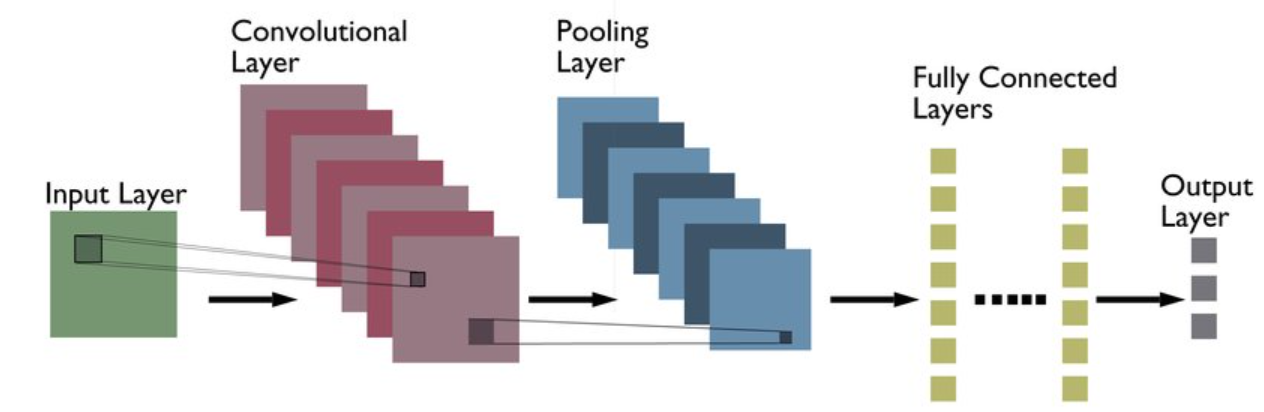
The following are definitions of different layers shown in the above architecture:
Convolutional layers
Convolutional layers operate by sliding a set of ‘filters’ or ‘kernels’ across the input data. Each filter is designed to detect a specific feature or pattern, such as edges, corners, or more complex shapes in the case of deeper layers. As these filters move across the image, they generate a map that signifies the areas where those features were found. The output of the convolutional layer is a feature map, which is a representation of the input image with the filters applied. Convolutional layers can be stacked to create more complex models, which can learn more intricate features from images. Simply speaking, convolutional layers are responsible for extracting features from the input images. These features might include edges, corners, textures, or more complex patterns.
Pooling layers
Pooling layers follow the convolutional layers and are used to reduce the spatial dimension of the input, making it easier to process and requiring less memory. In the context of images, “spatial dimensions” refer to the width and height of the image. An image is made up of pixels, and you can think of it like a grid, with rows and columns of tiny squares (pixels). By reducing the spatial dimensions, pooling layers help reduce the number of parameters or weights in the network. This helps to combat overfitting and help train the model in a fast manner. Max pooling helps in reducing computational complexity owing to reduction in size of feature map, and, making the model invariant to small transitions. Without max pooling, the network would not gain the ability to recognize features irrespective of small shifts or rotations. This would make the model less robust to variations in object positioning within the image, possibly affecting accuracy.
There are two main types of pooling: max pooling and average pooling. Max pooling takes the maximum value from each feature map. For example, if the pooling window size is 2×2, it will pick the pixel with the highest value in that 2×2 region. Max pooling effectively captures the most prominent feature or characteristic within the pooling window. Average pooling calculates the average of all values within the pooling window. It provides a smooth, average feature representation.
Fully connected layers
Fully-connected layers are one of the most basic types of layers in a convolutional neural network (CNN). As the name suggests, each neuron in a fully-connected layer is Fully connected- to every other neuron in the previous layer. Fully connected layers are typically used towards the end of a CNN- when the goal is to take the features learned by the convolutional and max pooling layers and use them to make predictions such as classifying the input to a label. For example, if we were using a CNN to classify images of animals, the final Fully connected layer might take the features learned by the previous layers and use them to classify an image as containing a dog, cat, bird, etc.
Fully connected layers take the high-dimensional output from the previous convolutional and pooling layers and flatten it into a one-dimensional vector. This allows the network to combine and integrate all the extracted features across the entire image, rather than considering localized features. It helps in understanding the global context of the image. The fully connected layers are responsible for mapping the integrated features to the desired output, such as class labels in classification tasks. They act as the final decision-making part of the network, determining what the extracted features mean in the context of the specific problem (e.g., recognizing a cat or a dog).
The combination of Convolution layer followed by max-pooling layer and then similar sets creates a hierarchy of features. The first layer detects simple patterns, and subsequent layers build on those to detect more complex patterns.
Output Layer
The output layer in a Convolutional Neural Network (CNN) plays a critical role as it’s the final layer that produces the actual output of the network, typically in the form of a classification or regression result. Its importance can be outlined as follows:
-
Transformation of Features to Final Output: The earlier layers of the CNN (convolutional, pooling, and fully connected layers) are responsible for extracting and transforming features from the input data. The output layer takes these high-level, abstracted features and transforms them into a final output form, which is directly interpretable in the context of the problem being solved.
-
Task-Specific Formulation:
- For classification tasks, the output layer typically uses a softmax activation function, which converts the input from the previous layers into a probability distribution over the predefined classes. The softmax function ensures that the output probabilities sum to 1, making them directly interpretable as class probabilities.
- For regression tasks, the output layer might consist of one or more neurons with linear or no activation function, providing continuous output values.
Real-world usage of CNN
CNNs are often used for image recognition and classification tasks. For example, CNNs can be used to identify objects in an image or to classify an image as being a cat or a dog. CNNs can also be used for more complex tasks, such as generating descriptions of an image or identifying the points of interest in an image. Beyond image data, CNNs can also handle time-series data, such as audio data or even text data, although other types of networks like Recurrent Neural Networks (RNNs) or transformers are often preferred for these scenarios. CNNs are a powerful tool for deep learning, and they have been used to achieve state-of-the-art results in many different applications.
Different types of CNN Architectures
The following is a list of different types of CNN architectures in deep learning that are most famous / popular ones:
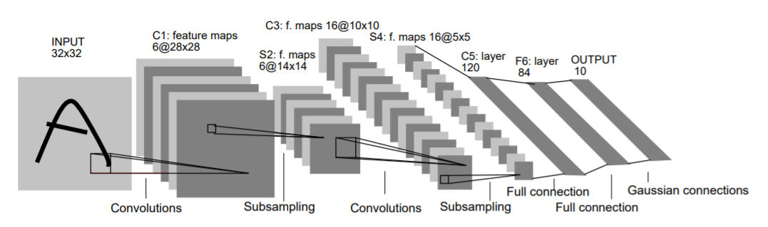
LeNet – First CNN Architecture
LeNet was developed in 1998 by Yann LeCun, Corinna Cortes, and Christopher Burges for handwritten digit recognition problems. LeNet was one of the first successful CNNs and is often considered the “Hello World” of deep learning. It is one of the earliest and most widely-used CNN architectures and has been successfully applied to tasks such as handwritten digit recognition. The LeNet architecture consists of multiple convolutional and pooling layers, followed by a fully-connected layer. The model has five convolution layers followed by two fully connected layers. LeNet was the beginning of CNNs in deep learning for computer vision problems. However, LeNet could not train well due to the vanishing gradients problem. To solve this issue, a shortcut connection layer known as max-pooling is used between convolutional layers to reduce the spatial size of images which helps prevent overfitting and allows CNNs to train more effectively. The diagram below represents LeNet-5 architecture.
The LeNet CNN is a simple yet powerful model that has been used for various tasks such as handwritten digit recognition, traffic sign recognition, and face detection. Although LeNet was developed more than 20 years ago, its architecture is still relevant today and continues to be used.
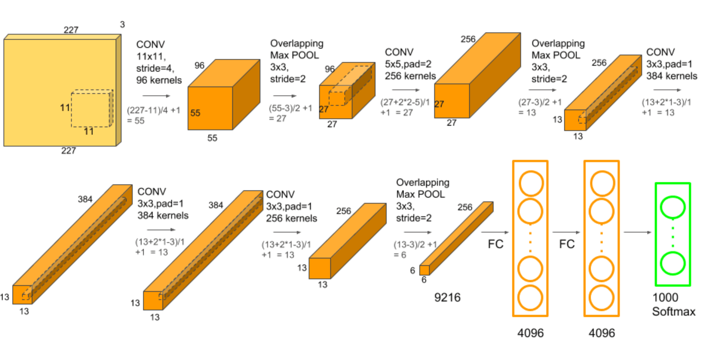
AlexNet – Deep Learning Architecture that popularized CNN
AlexNet was developed by Alex Krizhevsky, Ilya Sutskever, and Geoff Hinton. AlexNet network had a very similar architecture to LeNet, but was deeper, bigger, and featured Convolutional Layers stacked on top of each other. AlexNet was the first large-scale CNN and was used to win the ImageNet Large Scale Visual Recognition Challenge (ILSVRC) in 2012. The AlexNet architecture was designed to be used with large-scale image datasets and it achieved state-of-the-art results at the time of its publication. AlexNet is composed of 5 convolutional layers with a combination of max-pooling layers, 3 fully connected layers, and 2 dropout layers. The activation function used in all layers is Relu. The activation function used in the output layer is Softmax. The total number of parameters in this architecture is around 60 million.
ZF Net: ZFnet is the CNN architecture that uses a combination of fully-connected layers and CNNs. ZF Net was developed by Matthew Zeiler and Rob Fergus. It was the ILSVRC 2013 winner. The network has relatively fewer parameters than AlexNet, but still outperforms it on ILSVRC 2012 classification task by achieving top accuracy with only 1000 images per class. It was an improvement on AlexNet by tweaking the architecture hyperparameters, in particular by expanding the size of the middle convolutional layers and making the stride and filter size on the first layer smaller. It is based on the Zeiler and Fergus model, which was trained on the ImageNet dataset. ZF Net CNN architecture consists of a total of seven layers: Convolutional layer, max-pooling layer (downscaling), concatenation layer, convolutional layer with linear activation function, and stride one, dropout for regularization purposes applied before the fully connected output. This CNN model is computationally more efficient than AlexNet by introducing an approximate inference stage through deconvolutional layers in the middle of CNNs. Here is the paper on ZFNet.
GoogLeNet – CNN Architecture used by Google
GoogLeNet is the CNN architecture used by Google to win ILSVRC 2014 classification task. It was developed by Jeff Dean, Christian Szegedy, Alexandro Szegedy et al.. It has been shown to have a notably reduced error rate in comparison with previous winners AlexNet (Ilsvrc 2012 winner) and ZF-Net (Ilsvrc 2013 winner). In terms of error rate, the error is significantly lesser than VGG (2014 runner up). It achieves deeper architecture by employing a number of distinct techniques, including 1×1 convolution and global average pooling. GoogleNet CNN architecture is computationally expensive. To reduce the parameters that must be learned, it uses heavy unpooling layers on top of CNNs to remove spatial redundancy during training and also features shortcut connections between the first two convolutional layers before adding new filters in later CNN layers. Real-world applications/examples of GoogLeNet CNN architecture include Street View House Number (SVHN) digit recognition task, which is often used as a proxy for roadside object detection. Below is the simplified block diagram representing GoogLeNet CNN architecture:

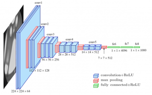
VGGNet – CNN Architecture with Large Filters
VGGNet is the CNN architecture that was developed by Karen Simonyan, Andrew Zisserman et al. at Oxford University. The full form of “VGG16” stands for “Visual Geometry Group 16“. This name comes from the Visual Geometry Group at the University of Oxford, where this neural network architecture was developed. The “16” in the name indicates that the model contains 16 layers that have weights; this includes convolutional layers as well as fully connected layers.
VGGNet is a 16-layer CNN with up to 95 million parameters and trained on over one billion images (1000 classes). It can take large input images of 224 x 224-pixel size for which it has 4096 convolutional features. CNNs with such large filters are expensive to train and require a lot of data, which is the main reason why CNN architectures like GoogLeNet (AlexNet architecture) work better than VGGNet for most image classification tasks where input images have a size between 100 x 100-pixel and 350 x 350 pixels. Real-world applications/examples of VGGNet CNN architecture include the ILSVRC 2014 classification task, which was also won by GoogleNet CNN architecture. The VGG CNN model is computationally efficient and serves as a strong baseline for many applications in computer vision due to its applicability for numerous tasks including object detection. Its deep feature representations are used across multiple neural network architectures like YOLO, SSD, etc. The diagram below represents the standard VGG16 network architecture diagram:

ResNet – CNN architecture that also got used for NLP tasks apart from Image Classification
ResNet is the CNN architecture that was developed by Kaiming He et al. to win the ILSVRC 2015 classification task with a top-five error of only 15.43%. The network has 152 layers and over one million parameters, which is considered deep even for CNNs because it would have taken more than 40 days on 32 GPUs to train the network on the ILSVRC 2015 dataset. CNNs are mostly used for image classification tasks with 1000 classes, but ResNet proves that CNNs can also be used successfully to solve natural language processing problems like sentence completion or machine comprehension, where it was used by the Microsoft Research Asia team in 2016 and 2017 respectively. Real-life applications/examples of ResNet CNN architecture include Microsoft’s machine comprehension system, which has used CNNs to generate the answers for more than 100k questions in over 20 categories. The CNN architecture ResNet is computationally efficient and can be scaled up or down to match the computational power of GPUs.
MobileNets – CNN Architecture for Mobile Devices
MobileNets are CNNs that can be fit on a mobile device to classify images or detect objects with low latency. MobileNets have been developed by Andrew G Trillion et al.. They are usually very small CNN architectures, which makes them easy to run in real-time using embedded devices like smartphones and drones. The architecture is also flexible so it has been tested on CNNs with 100-300 layers and it still works better than other architectures like VGGNet. Real-life examples of MobileNets CNN architecture include CNNs that is built into Android phones to run Google’s Mobile Vision API, which can automatically identify labels of popular objects in images.
ZFNet – Improved Version of AlexNet CNN Architecture
ZFNet, short for Zeiler and Fergus Network, is a convolutional neural network (CNN) model that gained significant attention in the field of deep learning, particularly in computer vision. It was developed by Matthew Zeiler and Rob Fergus and became well-known after winning the ImageNet Large Scale Visual Recognition Challenge (ILSVRC) in 2013.
The key innovation of ZFNet lies in its approach to improving the AlexNet architecture, which was the winner of the ILSVRC in 2012. ZFNet addressed some of the limitations of AlexNet by tweaking the CNN architecture, particularly focusing on the convolutional layers. ZFNet modified the first few layers of AlexNet. It used smaller filter sizes in the first and second convolutional layers and altered the stride and filter sizes to improve feature extraction. One of the most notable contributions of ZFNet was the introduction of a novel visualization technique that allowed for better understanding and interpretation of the feature maps in CNNs. By fine-tuning the architecture, ZFNet achieved improved performance in image classification tasks compared to its predecessor, AlexNet.
GoogLeNet_DeepDream – Generate images based on CNN features
GoogLeNet_DeepDream is a deep dream CNN architecture that was developed by Alexander Mordvintsev, Christopher Olah, et al.. It uses the Inception network to generate images based on CNN features. The architecture is often used with the ImageNet dataset to generate psychedelic images or create abstract artworks using human imagination at the ICLR 2017 workshop by David Ha, et al.
To summarize the different types of CNN architectures described above in an easy to remember form, you can use the following:
| Architecture | Year | Key Features | Use Case |
|---|---|---|---|
| LeNet | 1998 | First successful applications of CNNs, 5 layers (alternating between convolutional and pooling), Used tanh/sigmoid activation functions | Recognizing handwritten and machine-printed characters |
| AlexNet | 2012 | Deeper and wider than LeNet, Used ReLU activation function, Implemented dropout layers, Used GPUs for training | Large-scale image recognition tasks |
| ZFNet | 2013 | Similar architecture to AlexNet, but with different filter sizes and numbers of filters, Visualization techniques for understanding the network | ImageNet classification |
| VGGNet | 2014 | Deeper networks with smaller filters (3×3), All convolutional layers have the same depth, Multiple configurations (VGG16, VGG19) | Large-scale image recognition |
| ResNet | 2015 | Introduced “skip connections” or “shortcuts” to enable training of deeper networks, Multiple configurations (ResNet-50, ResNet-101, ResNet-152) | Large-scale image recognition, won 1st place in the ILSVRC 2015 |
| GoogleLeNet | 2014 | Introduced Inception module, which allows for more efficient computation and deeper networks, multiple versions (Inception v1, v2, v3, v4) | Large-scale image recognition, won 1st place in the ILSVRC 2014 |
| MobileNets | 2017 | Designed for mobile and embedded vision applications, Uses depthwise separable convolutions to reduce the model size and complexity | Mobile and embedded vision applications, real-time object detection |
CNN Architecture for Image Classification: Python Code Example
The following Python code demonstrates how to use a simple Convolutional Neural Network (CNN) to classify images from the sklearn digits dataset using TensorFlow and Keras. The digits dataset This dataset contains 8×8 pixel images of handwritten digits (0 through 9), which is a good size for a simple CNN demonstration. Here is a brief overview of digits dataset:
- Dataset Characteristics: 1,797 samples of 8×8 images, each representing a handwritten digit.
- Target Classes: 10 (digits from 0 to 9).
- Image Size: 8×8 pixels.
Although the digits dataset is relatively simple and small, especially compared to typical datasets used for CNNs (like MNIST or CIFAR-10), it can still be useful for illustrating the basic principles of how a CNN works.
Note that the performance of a CNN on such a small and simple dataset may not be as impressive or illustrative as it would be on larger, more complex datasets. For more advanced or realistic demonstrations of CNN capabilities, datasets like MNIST (handwritten digits), CIFAR-10 (60,000 32×32 color images in 10 classes), or ImageNet (large dataset for more complex image recognition tasks) are generally preferred.
The following steps are used for training the CNN model:
- Load the digits dataset.
- Preprocess the data: This includes normalizing the pixel values and reshaping the images to the format expected by the CNN.
- Build a simple CNN model.
- Compile the model, specifying the loss function and optimizer.
- Train the model on the digits data.
- Evaluate the model’s performance.
from sklearn.datasets import load_digits
from sklearn.model_selection import train_test_split
from tensorflow.keras.utils import to_categorical
from tensorflow.keras.models import Sequential
from tensorflow.keras.layers import Dense, Conv2D, Flatten, MaxPooling2D

# Load the digits dataset
digits = load_digits()
X, y = digits.images, digits.target

# Preprocessing
# Normalizing pixel values
X = X / 16.0

# Reshaping the data to fit the model
# CNN in Keras requires an extra dimension at the end for channels,
# and the digits images are grayscale so it's just 1 channel
X = X.reshape(-1, 8, 8, 1)

# Convert labels to categorical (one-hot encoding)
y = to_categorical(y)

# Splitting into training and testing sets
X_train, X_test, y_train, y_test = train_test_split(X, y, test_size=0.2, random_state=42)

# Building a simple CNN model
model = Sequential()
model.add(Conv2D(64, kernel_size=3, activation='relu', input_shape=(8, 8, 1)))
model.add(MaxPooling2D(pool_size=(2, 2)))
model.add(Flatten())
model.add(Dense(50, activation='relu'))
model.add(Dense(10, activation='softmax'))  # 10 classes for digits 0-9

# Compiling the model
model.compile(optimizer='adam', loss='categorical_crossentropy', metrics=['accuracy'])

# Training the model
model.fit(X_train, y_train, validation_data=(X_test, y_test), epochs=10)

# Evaluate the model
accuracy = model.evaluate(X_test, y_test)[1]
print("Test accuracy:", accuracy)
Conclusion
Convolutional neural network has evolved from their inception with LeNet to the streamlined efficiency of MobileNets. Each architecture, from AlexNet to ResNet and beyond, has brought unique enhancements that have deepened our understanding and usage of CNNs. They have pushed the boundaries of what’s possible in image recognition and classification tasks, and have had widespread applications in various domains. he future of CNNs holds exciting opportunities and challenges, promising to further transform our digital landscape. Should you have any questions or require further understanding, please don’t hesitate to reach out. I will be happy to help you navigate and learn in a better manner.

Check out my latest book titled as First Principles Thinking: Building winning products using first principles thinking.
- Mathematics Topics for Machine Learning Beginners - July 6, 2025
- Questions to Ask When Thinking Like a Product Leader - July 3, 2025
- Three Approaches to Creating AI Agents: Code Examples - June 27, 2025
I found it very helpful. However the differences are not too understandable for me