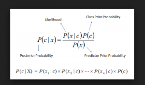
In this post, you will learn about the difference between Frequentist vs Bayesian Probability. It is of utmost importance to understand these concepts if you are getting started with Data Science.
What is Frequentist Probability?
Probability is used to represent and reason about uncertainty. It was originally developed to analyze the frequency of the events. In other words, the probability was developed as frequentist probability.
The probability of occurrence of an event, when calculated as a function of the frequency of the occurrence of the event of that type, is called Frequentist Probability. Frequentist probability is a way of assigning probabilities to events that take into account how often those events actually occur. Frequentist probability is sometimes also called objective probability or empirical probability. For example, the probability of rolling a dice (having 1 to 6 numbers) and getting a number 3 can be said to be Frequentist probability. Consider another example of a head occurring as a result of tossing a coin.
The Frequentist frequencies can be calculated by conducting the experiment in a repetitive manner for infinite times or possibly a large number of times and calculating the probability by counting the number of times an event of a particular type occurred.
However, in real-world scenarios which are not repeatable, frequentist probability won’t hold well. This is where Bayesian probability comes into the picture.
What is Bayesian Probability?
The probability of the occurrence of an event when calculated based on the degree of belief (based on the prior knowledge) is called the Bayesian probability. Such events do not fall under repetitive kinds of events. For example, let’s say a civil engineer is asked about the likelihood or probability of a flyover bridge crashing down in the coming rainy season. The civil engineer would be able to speak about the chances based on his/her degree of belief (vis-a-vis data made available to him about the life of the bridge, construction material used, etc). This is because events such as the falling of the flyover bridge can’t be repeated multiple times (doesn’t make sense in the first place) to calculate the probability or chance. In another example, if a doctor after seeing the patient’s report says that there are 40% chance of a patient suffering from a disease, it is the degree of belief that is represented as the probability (Bayesian) and not that with a large no. of patients, 40% will have that disease.
Mathematically, a Bayesian probability is calculated using the Bayes Rule formula which is used for determining how strongly a set of evidence supports the hypothesis. In other words, it is used to calculate the conditional probability of a given hypothesis given a set of evidence. Given the hypothesis is H, and the evidence is E, the fact related to how strongly the hypothesis H is supported by evidence E can be calculated as P(H/E). The following is the formula of the Bayes Rule.

Fig 1. Bayesian Probability – Bayes Rule
In the above formula,
-
P(H/E) is the probability of hypothesis H to take place (or, H is true) given that the evidence E happened (or, E is true). It is also termed as Posterior Probability of Hypothesis, H.
-
P(H) is the probability of the hypothesis before learning about the evidence E. It is also called as Prior Probability of Hypothesis H.
-
P(E/H) is the likelihood that the evidence E is true or happened given that hypothesis H is true.
-
P(E) is the probability of the evidence E to occur irrespective of whether hypothesis H is true or false. It is also called the total probability of the evidence.
Using the above example, the Bayesian probability can be articulated as the probability of a flyover bridge crashing down given it is built 25 years back. It can also be read as to how strongly the evidence that the flyover bridge is built 25 years back, supports the hypothesis that the flyover bridge would come crashing down. Here the hypothesis is that “the flyover bridge crashes down” (let’s call it BRIDGE_CRASHING_DOWN) and the evidence or supporting facts is “the flyover bridge is built 25 years back” (let’s call it BRIDGE_BUILT_25_YEARS_BACK).
The Bayesian probability can be defined as P(BRIDGE_CRASHING_DOWN / BRIDGE_BUILT_25_YEARS_BACK).

Fig 2. Bayesian Probability Example
It could be read as the following:
-
P(BRIDGE_CRASHING_DOWN) is the probability of the bridge crashing down even before the evidence such as the age of the bridge was known.
-
P(BRIDGE_BUILT_25_YEARS_BACK/BRIDGE_CRASHING_DOWN) is the probability that a bridge is found to be built 25 years back given that bridge came crashing down.
-
P(BRIDGE_BUILT_25_YEARS_BACK) is the probability that the bridge is built 25 years back.
References
Summary
In this post, you learned about what is Frequentist Probability and Bayesian Probability with examples and their differences.
Did you find this article useful? Do you have any questions or suggestions about this article? Leave a comment and ask your questions and I shall do my best to address your queries.
- Three Approaches to Creating AI Agents: Code Examples - June 27, 2025
- What is Embodied AI? Explained with Examples - May 11, 2025
- Retrieval Augmented Generation (RAG) & LLM: Examples - February 15, 2025
I found it very helpful. However the differences are not too understandable for me