
Descriptive statistics is a branch of statistics that deals with the analysis of data. It is concerned with summarizing and describing the characteristics of a dataset. It is one of the most fundamental tool for data scientists to understand the data as they get started working on the dataset. In this blog post, I will cover the key concepts of descriptive statistics, including measures of central tendency, measures of spread and statistical moments.
What’s Descriptive Statistics & Why do we need it?
Descriptive statistics is used to summarize and describe the characteristics of a dataset in terms of understanding its mean & related measures, spread or dispersion of the data around the mean, etc. The following are some of the important reasons why we need descriptive statistics in the first place:
- Simplifying complex dataset: It helps us simplify the complex data by summarizing its key characteristics (using measures of central tendency or spread / dispersion), making it easier to understand and interpret.
- Data comparison: It helps us compare the data from different perspectives including its central tendency and spread / dispersion measures.
- Making predictions: It does help with making predictions based on measure of central tendency. For example, let’s say we want to predict the future price of a particular stock based on its historical prices. By calculating the mean or median price of the stock over a given period, we can identify the central tendency around which the prices are clustered. This can be used as a baseline for predicting future prices. If the future prices are significantly higher or lower than the central tendency, this could indicate a change in the underlying factors affecting the stock price. Another example includes usage of measures of spread such as variance or standard deviation. Let’s say we want to predict the future sales of a particular product based on its historical sales data. By calculating the variance or standard deviation of the sales data, we can identify the level of variability in the sales figures. This can be used to adjust your predictions and take into account any potential fluctuations in sales.
- Decision making: It can help with decision-making in several ways by leveraging measures of central tendency and spread. For example, let’s say we want to make a decision about pricing a new product. By analyzing the prices of similar products in the market and calculating the mean price and its spread (variance / standard deviation), we can identify the typical price range for similar products. This information can be used to make a decision about the price of your new product, such as whether to price it within or outside the typical price range.
Key Components of Descriptive Statistics
Now that we understand what descriptive statistics is and why it is important, let’s take a closer look at some of its key components. These components include measures of central tendency, measures of dispersion, and statistical moments. By understanding these components, we can gain a more detailed understanding of the characteristics of a dataset, which can be used to make informed decisions and predictions based on data.
Measures of Central Tendency
Measures of central tendency can be defined as statistical measures that provide information about the typical or central value of a dataset. They are used to summarize the data by identifying the central point around which the data is clustered. The three most commonly used measures of central tendency are:
- Mean: The mean is the sum of all values in the dataset divided by the number of values. It is the arithmetic average of the dataset.
- Median: The median is the middle value of a dataset when the values are arranged in order. If the dataset has an even number of values, the median is the average of the two middle values.
- Mode: The mode is the value that appears most frequently in the dataset.
The following represents some mathematical examples that would help understand the concepts of mean, median, and mode:
- Mean: Let’s say we have a dataset of five numbers: 2, 4, 6, 8, and 10. To calculate the mean, we add up all the numbers and divide by the total number of values:(2 + 4 + 6 + 8 + 10) / 5 = 6. Therefore, the mean of this dataset is 6.
- Median: Let’s use the same dataset of five numbers: 2, 4, 6, 8, and 10. To calculate the median, we first arrange the numbers in ascending order:2, 4, 6, 8, 10. The median is the middle value of the dataset. Since there are an odd number of values, the median is simply the middle value, which is 6 in this case. In case the number of values is even, the median value is calculated as the average of the two middle values in the dataset. To do this, we first arrange the values in ascending or descending order, then take the mean of the two middle values. For example, if we have the dataset 2, 4, 6, 8, the two middle values are 4 and 6, so the median value is (4 + 6) / 2 = 5.
- Mode: Let’s say we have a dataset of ten numbers: 2, 3, 3, 5, 5, 5, 6, 7, 7, and 8. To calculate the mode, we identify the value that appears most frequently in the dataset. In this case, the value 5 appears three times, which is more than any other value in the dataset. Therefore, the mode of this dataset is 5.
It is important to note that measures of central tendency can be affected by outliers or skewed data, which can lead to misleading results. Therefore, it is often useful to use measures of dispersion in combination with measures of central tendency to gain a more complete understanding of the dataset.
Measures of Spread or Dispersion
Measures of spread or dispersion can be defined as statistical measures that provide information about the variability or spread of a dataset. They are used to describe how far apart the values in a dataset are from each other and from the central value. Measures of spread are important because they can provide insights into the level of uncertainty or variability in the data. Some of the commonly used measures of spread include range, interquartile range, variance, and standard deviation
Variance
Variance is one of the most important concepts as a measure of spread. It is defined as the average of the squared differences between each value in the dataset and the mean of the dataset. In other words, it measures how far each value in the dataset is from the mean, on average.
The formula for variance is:
[latex]\operatorname{Var}(X) = \frac{1}{n-1}\sum_{i=1}^{n}(X_i – \bar{X})^2[/latex]
Where [latex]\operatorname{Var}(X)[/latex] represents the variance of the variable [latex]X[/latex], [latex]n[/latex] represents the sample size, [latex]X_i[/latex] represents the [latex]i[/latex]th observation in the sample, [latex]\bar{X}[/latex] represents the sample mean, and the symbol [latex]\sum[/latex] represents the sum of the terms inside the parentheses. The resulting value of variance is always positive or zero. A higher variance indicates that the data points are more spread out from the mean, while a lower variance indicates that the data points are closer to the mean.
Standard Deviation
Standard deviation is another key concept as a measure of spread. It is defined as the square root of the variance. In other words, it measures the amount of dispersion or spread of the data points from the mean. Standard deviation is expressed in the same units as the original data, making it a useful measure for comparing datasets with different scales. The formula for standard deviation for a sample is:
Standard Deviation = [latex]\sqrt{\frac{\sum_{i=1}^{n}(x_i – \bar{x})^2}{n-1}}[/latex]
where [latex]x_i[/latex] represents each value in the dataset, [latex]\bar{x}[/latex] represents the mean of the dataset, and [latex]n[/latex] represents the number of values in the dataset. In case, you want to find the standard deviation of population, it is [latex]N[/latex]. Standard deviation is a commonly used measure of spread in statistical analysis and modeling, and is often used in conjunction with the mean to summarize and describe the characteristics of a dataset.
Range
Range is another measure of spread which determines the difference between the largest and smallest values in a dataset. It provides a simple measure of how spread out the data.
The formula for range is:
Range = Maximum value – Minimum value
Where the maximum value is the largest value in the dataset and the minimum value is the smallest value in the dataset. Range is a useful measure of spread for datasets with a small number of values or for providing a quick overview of the variability in the data. However, it does not provide as much information as other measures of spread such as variance or standard deviation.
Interquartile Range (IQR)
Interquartile range (IQR) is another measure of spread which is used to describe the spread of the middle 50% of the data in a dataset. It is calculated by finding the difference between the third quartile (Q3) and the first quartile (Q1), which represent the 75th and 25th percentiles of the dataset, respectively. The formula for IQR is:
IQR = Q3 – Q1
The IQR is a useful measure of spread for datasets that contain outliers or are skewed, as it focuses on the middle portion of the data and is less affected by extreme values. The IQR can also be used to identify potential outliers in the data, as values that fall outside of the range of 1.5 times the IQR above or below the upper or lower quartile are often considered to be outliers.
Statistical Moments
Statistical moments is another key concept in descriptive statistics which are used to describe the shape and characteristics of the data distribution. A moment is a quantitative measure of a distribution, and the moments of a distribution are used to calculate various statistical properties such as the mean, variance, skewness, and kurtosis.
The formula for the nth statistical moment of a continuous probability distribution is:
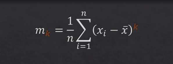
In the above formula, the k represents kth moment. By replacing the value of k with 1, 2, 3, 4 we can find first moment, second moment, third moment and fourth moment. The following is how different moments will look like:
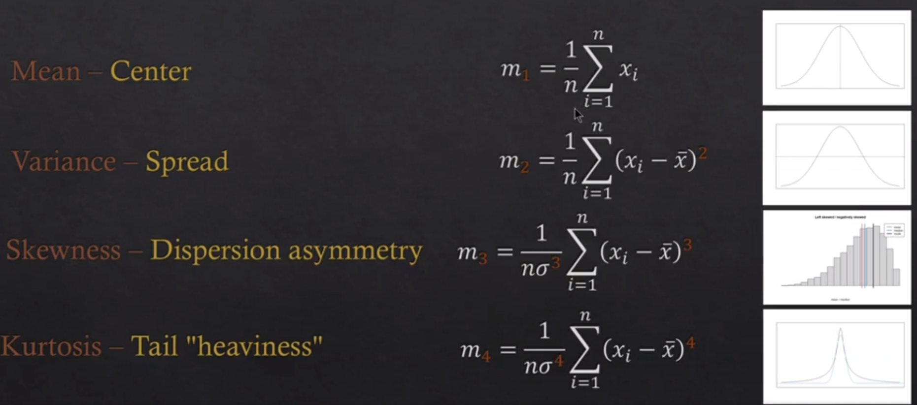
We have understood the concepts of mean and variance as measure of central tendency and measure of spread / dispersion. Here is the concept of skewness and kurtosis:
Skewness
Skewness can be defined as the statistical moment which represents the degree of asymmetry of a probability distribution around its mean. Specifically, skewness measures the lack of symmetry in the tails of the distribution, with positive skewness indicating a longer or fatter tail on the positive side or right side and negative skewness indicating a longer or fatter tail on the negative side or left side. The following picture shows the right tailed (positive) and left-tailed (negative) skewed distribution.
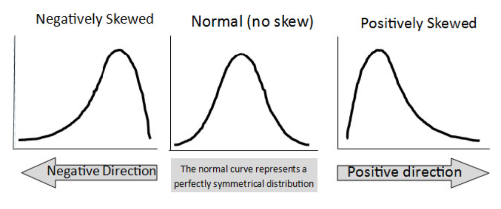
The value of skewness can be positive or negative. The positive value would mean that the tail of the data distribution is skewed towards the right, or the positive side of the distribution as per the above diagram. This indicates that there are more extreme values on the positive side than on the negative side, and the mean is likely to be larger than the median. On the other hand, a negative value of skewness means that the tail of the distribution is skewed towards the left, or the negative side of the distribution. This indicates that there are more extreme values on the negative side than on the positive side, and the mean is likely to be smaller than the median. A value of zero for skewness indicates a perfectly symmetrical distribution (normal distribution).
Kurtosis
Kurtosis can be defined as the statistical moment which represents the degree of tail heaviness of a probability distribution relative to a normal distribution. Specifically, kurtosis measures the extent to which the tails of a distribution differ from those of a normal distribution. The distribution with high value of kurtosis would mean that the distribution has heavier tails than a normal distribution. This is often referred to as a leptokurtic distribution. A high kurtosis indicates that there are more extreme values in the tails of the distribution than would be expected for a normal distribution. Examples of leptokurtic distributions include the Student’s t-distribution, Rayleigh distribution, Laplace distribution, exponential distribution, Poisson distribution, etc. On the other hand, a distribution with low kurtosis has lighter tails than a normal distribution. This is often referred to as a platykurtic distribution. A low kurtosis indicates that there are fewer extreme values in the tails of the distribution than would be expected for a normal distribution. Examples of platykurtic distributions include continuous and discrete uniform distributions. These distributions have a negative kurtosis, which means that they have thinner tails than the normal distribution.
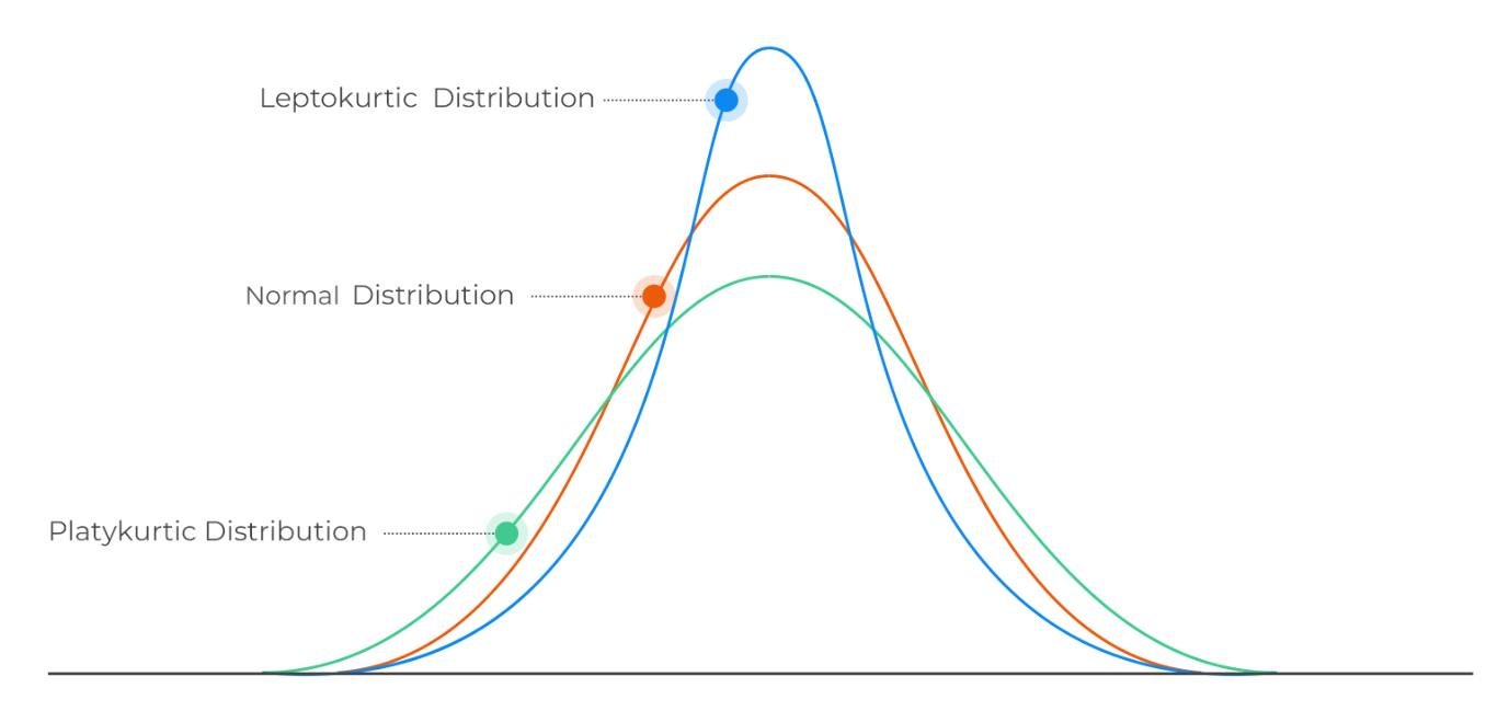
A normal distribution (mesokurtic) has a kurtosis of 0, so any distribution with a kurtosis greater than 0 is considered to be leptokurtic, while any distribution with a kurtosis less than 0 is considered to be platykurtic.
Conclusion
Descriptive statistics is an important tool for summarizing and describing the characteristics of a dataset. It provides a set of measures that are used to describe the central tendency, spread, and shape of the data. In this article, we have covered some of the key concepts of descriptive statistics, including measures of central tendency, measures of dispersion or spread, and statistical moments.
Measures of central tendency, such as mean, median, and mode, provide information about the center of the data and are useful for summarizing the overall characteristics of the dataset. Measures of dispersion or spread, such as range, interquartile range, variance, and standard deviation, provide information about the variability or spread of the data and are useful for identifying any potential outliers or patterns in the data. Statistical moments, such as skewness and kurtosis, provide information about the shape of the distribution and are useful for characterizing the properties of the data.
Understanding these key concepts of descriptive statistics is important for data scientists, as it enables them to analyze and interpret data more effectively. By using measures of central tendency, dispersion, and statistical moments, data scientists can gain valuable insights into the data and make informed decisions based on the characteristics of the dataset. Whether you are working in finance, engineering, or any other field that involves data analysis, a solid understanding of descriptive statistics is essential for success.

Check out my latest book titled as First Principles Thinking: Building winning products using first principles thinking.
- Mathematics Topics for Machine Learning Beginners - July 6, 2025
- Questions to Ask When Thinking Like a Product Leader - July 3, 2025
- Three Approaches to Creating AI Agents: Code Examples - June 27, 2025
Low kurtosis does not imply a flatter peak. For example, the beta(.5,1) distribution is infinitely peaked but has low kurtosis.
Thank you Peter. The comment was indeed very insightful. Made the changes to the content.