Chebyshev’s theorem is a fundamental concept in statistics that allows us to determine the probability of data values falling within a certain range defined by mean and standard deviation. This theorem makes it possible to calculate the probability of a given dataset being within K standard deviations away from the mean. It is important for data scientists, statisticians, and analysts to understand this theorem as it can be used to assess the spread of data points around a mean value.
What is Chebyshev’s Theorem?
Chebyshev’s Theorem, also known as Chebyshev’s Rule, states that in any probability distribution, the proportion of outcomes that lie within k standard deviations from the mean is at least 1 – 1/k², for any k greater than 1. This theorem is also called Chebyshev’s inequality.
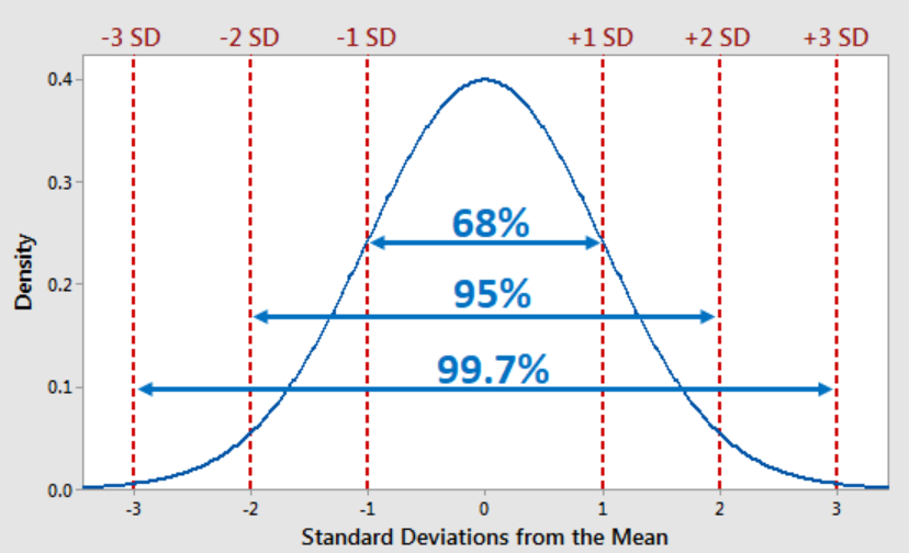
The Chebyshev’s rule can be applied to all distributions regardless of their shape and can be used whenever the data distribution shape is unknown or is non normal. If the data distribution is known as normal distribution, one can apply the empirical rule (68-95-99.7) which looks like the following and states that given normal data distribution, 68% of the data falls within 1 standard deviation, 95% of data falls within two standard deviation and 99.7 % of data falls within 3 standard deviations.
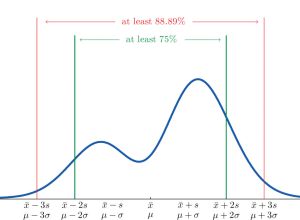
As per Chebyshev’s theorem, at least $1 – \frac{1}{k^2}$ values will fall within ±k standard deviations of the mean regardless of the shape of the distribution for values of k > 1. This looks like the following when plotted. The plot represents that 75% of values will fall under 2 standard deviations of mean and 88.88% of values will fall within 3 standard deviations of the mean.
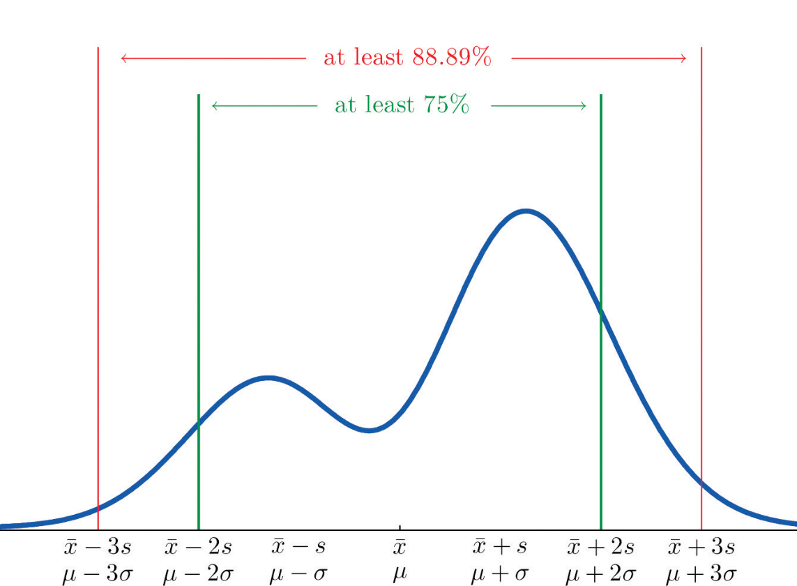
75% is calculated as 1 − 1/k2 = 1 − 1/22 = 3/4 = .75. Note the value of k = 2. When comparing with the empirical rule if the data are normally distributed, 95% of all values are within μ ± 2σ (2 standard deviations). Similarly, the percentage of values within 3 standard deviations of the mean is at least 89%, in contrast to 99.7% for the empirical rule.
Chebyshev’s Rule Formula
The Chebyshev’s theorem or Chebyshev’s inequality formula looks like the following:
$P(|X – \mu| \geq k\sigma) \leq \frac{1}{k^2}$
where:
- P denotes probability,
- X is a random variable,
- μ is the mean of X,
- σ is the standard deviation of X,
- k is any positive number greater than 1,
- ∣X−μ∣ represents the absolute deviation of X from its mean μ,
- kσ is the distance from the mean, measured in units of standard deviation.
In simpler terms, this inequality tells us that for any distribution with a finite variance, the probability that a value will be more than k standard deviations away from the mean is at most $\frac{1}{k^2}$. Conversely, it also implies that the probability that a value is within k standard deviations of the mean is at least $1 – \frac{1}{k^2}$
Chebyshev’s Theorem Example
Let’s look at an example to better understand how Chebyshev’s theorem works in practice.
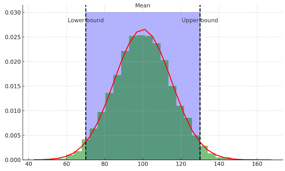
The plot above demonstrates Chebyshev’s inequality using a normal distribution as an example, which is a common real-world distribution for many natural and social phenomena.
In this plot:
- The green histogram represents the distribution of a population with a mean (μ) of 100 and a standard deviation (σ) of 15.
- The red curve is the probability density function for the normal distribution with the same mean and standard deviation.
- The dashed black lines represent the bounds within k standard deviations from the mean (in this case, k = 2).
- The blue shaded area between the dashed lines shows the data within 2 standard deviations of the mean.
According to Chebyshev’s inequality, at least $1 – \frac{1}{k^2}$ (which equals 75% for k=2) of the data should fall within 2 standard deviations of the mean. The plot demonstrates that the actual proportion of data within 2 standard deviations is indeed above this lower bound, as expected in a real-world scenario. The exact proportion within k standard deviations from the mean is calculated and shown on the plot, which in this case is higher than the Chebyshev’s lower bound due to the properties of the normal distribution.
Lets look at a real world example to understand Chebyshev’s rule in a better manner.
Problem: The number of daily downloads for a mobile app is a random variable with a mean (μ) of 50 and a standard deviation (σ) of 8. Find the probability with which we can assert that there will be more than 34 but less than 66 downloads in a day.
Solution: We want to find the probability that the number of downloads will be within k standard deviations of the mean, where k is determined by the range [μ – kσ, μ + kσ] that we are interested in. For our case, we are looking at the range from 34 to 66 downloads.
First, we calculate the value of k for both the lower and upper bounds:
- For the lower bound (more than 34 downloads):
50−k⋅8=34
k⋅8=50−34
k⋅8=16
k=2 - For the upper bound (less than 66 downloads):
50+k⋅8=66
k⋅8=66−50
k⋅8=16
k=2
Since k is the same for both bounds, we can use k = 2 to apply Chebyshev’s Theorem.
Now, we can apply Chebyshev’s inequality to find the minimum probability that the number of downloads will be between 34 and 66:
$P ≥ 1−\frac{1}{k^2}$
$P ≥ 1−\frac{1}{2^2}$
$P ≥ 1−\frac{1}{4}$
$P ≥ 0.75$
Therefore, we can assert with at least 75% probability that there will be more than 34 but less than 66 daily downloads of the mobile app.
Conclusion
In summary, Chebyshev’s theorem provides us with an easy way to calculate how many data points should fall within a certain range from their mean value based on their standard deviation and desired variance level if the data distribution is unknown or non-normal. This understanding can help us better assess where outliers may exist in our datasets and use this information for further analysis or predictions about our datasets’ behaviors over time. Whether you’re working with small or large datasets, having an understanding of Chebychev’s theorem can help you get more accurate insights into your data!

Check out my latest book titled as First Principles Thinking: Building winning products using first principles thinking.
- Three Approaches to Creating AI Agents: Code Examples - June 27, 2025
- What is Embodied AI? Explained with Examples - May 11, 2025
- Retrieval Augmented Generation (RAG) & LLM: Examples - February 15, 2025
I found it very helpful. However the differences are not too understandable for me