In this post, you will learn about Bayes’ Theorem with the help of examples. It is of utmost importance to get a good understanding of Bayes Theorem in order to create probabilistic models. Bayes’ theorem is alternatively called as Bayes’ rule or Bayes’ law. One of the many applications of Bayes’s theorem is Bayesian inference which is one of the approaches of statistical inference (other being Frequentist inference), and fundamental to Bayesian statistics. In this post, you will learn about the following:
- Introduction to Bayes’ Theorem
- Bayes’ theorem real-world examples
Introduction to Bayes’ Theorem
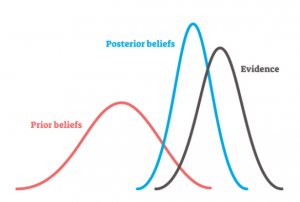
In simple words, Bayes Theorem is used to determine the probability of a hypothesis in the presence of more evidence or information. In other words, given the prior belief (expressed as prior probability) related to a hypothesis and the new evidence or data or information given the hypothesis is true, Bayes theorem help in updating the beliefs (posterior probability) related to hypothesis. Let’s represent this mathematically. Let’s understand this using a diagram given below:
In the above diagram, the prior beliefs is represented using red color probability distribution with some value for the parameters. In the light of data / information / evidence (given the hypothesis is true) represented using black color probability distribution, the beliefs gets updated resulting in different probability distribution (blue color) with different set of parameters. The updated belief is also called as posterior beliefs.
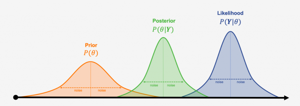
If the prior beliefs about the hypothesis is represented as P([latex]\theta[/latex]), and the information or data given the prior belief is represented as P([latex]Y | \theta[/latex]), then the posterior belief related to hypothesis can be represented as the following:
[latex]P(\theta | Y) \propto P(Y | \theta) * P(\theta)[/latex] … Eq 1
The above expression when applied with a normalisation factor also called as marginal likelihood (probability of observing the data averaged over all the possible values the parameters) can be written as the following:
[latex]P(\theta | Y) = \frac{P(Y | \theta) * P(\theta)}{P(Y)}[/latex]
The following is an explanation of different probability components in the above equation:
- Prior Probability P([latex]\theta[/latex]): The prior probability distribution represents the prior beliefs about the hypothesis.
- Likelihood P([latex]Y | \theta[/latex]): The Likelihood represents the evidence or information or data given the prior probability.
- Posterior Probability P([latex]\theta | Y[/latex]): The posterior probability distribution represents the updated beliefs about the hypothesis given the evidence (represented by likelihood distribution).
- Marginal Probability or Likelihood P([latex]Y[/latex]): The probability of observing the data / information under all possible hypotheses. Marginal probability can be represented as [latex]\sum P(Y | \theta_i)*P(\theta_i)[/latex]
Conceptually, the posterior can be thought of as the updated prior in the light of new evidence / data / information. As a matter of fact, the posterior belief / probability distribution from one analysis can be used as the prior belief / probability distribution for a new analysis. This makes Bayesian analysis suitable for analysing data that becomes available in sequential order.
Bayes’ Theorem Real-world Examples
Here are some real-world examples of Bayes’ Theorem:
- Healthcare: Application of Bayes’ Theorem can be found in the field of medicine involving uncertainty related to diagnosis, treatment selection and prediction of prognosis (possible outcomes of disease). Probabilistic models based on Bayes’ theorem can be used to help doctors in judging the diagnosis and selecting an appropriate treatment to address the diseases.
- Computer applications such as spam filters: Bayesian inference is used for creating a spam filter application used for classifying whether an email is spam or otherwise. The idea is to use the new evidence / data to update the existing beliefs (prior probability) about which email is spam or otherwise in order to have updated beliefs (posterior probability).
- Bioinformatics applications: Bayesian inference can be used to build applications in Bioinformatics domain such as differential gene expression analysis.
- Legal applications: Bayesian inference can be used by jurors to coherently accumulate the evidence for and against a defendant by applying Bayes’ theorem to all evidence presented, with the posterior from one stage becoming the prior for the next.
- Bayesian based search applications: Bayesian search theory can be applied to search for lost objects. Its application has been found in searching several lost sea vessels, flight recorders. Recently, Bayes theory was also applied to find missing Malaysian airlines flight 370.

Check out my latest book titled as First Principles Thinking: Building winning products using first principles thinking.
- Questions to Ask When Thinking Like a Product Leader - July 3, 2025
- Three Approaches to Creating AI Agents: Code Examples - June 27, 2025
- What is Embodied AI? Explained with Examples - May 11, 2025
I found it very helpful. However the differences are not too understandable for me