
Probability is a branch of mathematics that deals with the likelihood of an event occurring. It is important to understand probability concepts if you want to get good at data science and machine learning. In this blog post, we will discuss the basic concepts of probability and provide examples to help you understand it better. We will also introduce some common formulas associated with probability. So, let’s get started!
What is probability and what are the different types?
Probability is a concept in mathematics that measures the likelihood of an event occurring. It is typically expressed as a number between 0 and 1, with 0 indicating that an event is impossible and 1 indicating that an event is certain to occur or the event will always happen. The concept of probability can be used to model a variety of situations, from the roll of a dice to the probability of winning the lottery. Probability can be calculated using either theoretical or experimental methods. Theoretical probability is based on known rates and proportions, while experimental probability is based on actual data. Regardless of which method is used, probability can give us valuable insights into the likelihood of future events. Probability is an important tool for statisticians, mathematicians, scientists, and everyday people alike. By understanding probability, we can make better decisions, create more accurate predictions, and avoid potential pitfalls.
There are three types of probability:
- Experimental probability: This is the probability that an event will occur, based on experimental data. It is usually calculated by conducting a trial or experiment and observing the outcome. For example, if you flip a coin 10 times and it lands on heads six times, then the experimental probability of the coin landing on heads is 0.6. Experimental probability can be used to predict the likelihood of an event occurring in the future, based on past data. However, it is important to note that experimental probability is only an estimate, and actual results may vary.
- Theoretical probability: The theoretical probability is the likelihood of an event occurring, as calculated by taking the number of ways the event can occur and dividing it by the total number of possible outcomes. For example, if there are five equally likely outcomes and only one of them is the event in question, then the theoretical probability of the event happening is one out of five or 20%. The theoretical probability can be thought of as the long-term average of how often an event occurs, assuming that a large number of trials are conducted. It contrasts with actual probability, which is the likelihood of an event occurring based on observed data. While the theoretical probability is calculated using assumptions and theoretical models, the actual probability is based on empirical evidence. Nevertheless, theoretical probability can provide a useful estimate of how likely an event is to occur.
- Subjective probability: Subjective probability is based on an individual’s personal judgment or belief about the likelihood of an event occurring. It is not based on any mathematical calculation or observed data. For example, if you believe that there is a 50% chance of rain tomorrow, then your subjective probability of rain tomorrow is 0.50. Subjective probability is often used in situations where there is no experimental or theoretical data to rely on. For example, when making a decision about whether or not to buy insurance, people will often use their subjective probability of experiencing an event (e.g., getting into a car accident) to help them make their decision.
Before getting into understanding concepts, formulas, let’s understand some basic terminologies used in the probability related problems:
- Sample space: The set of all possible outcomes of a probability experiment is called the sample space. If an experiment represents tossing a coin once, the sample space representing all possible outcomes of the experiment consists of either head (H) or tail (T). Thus, sample space = {H, T}. If the experiment represents tossing the coin twice, the sample space = {HH, HT, TH, TT}. If tossing a single die once is an experiment, sample space = {1, 2, 3, 4, 5, 6} representing all possible outcomes. If the outcome is all possible even numbers, the sample space = {2, 4, 6}. If the outcome is all possible odd numbers, the sample space = {1, 3, 5}. An experiment can have different sample spaces based on types of all possible expected outcomes.
- Event: Any subset of the sample space is called an event. For example, for the experiment representing single toss coin, the sample space = {1, 2, 3, 4, 5, 6}. All possible outcomes which are even represent the event. Event is denoted by capital letter, A, B, C, etc. Thus, the event representing event outcomes = {2, 4, 6}
- Simple Event: An event that consists of a single outcome is called a simple event.
- Compound Event: An event that consists of two or more outcomes is called a compound event.
- Mutually Exclusive Events: Two events are said to be mutually exclusive if they cannot occur simultaneously.
- Random variable: Random variable represents variable that can take different values in a random manner with different probability. Random variable is denoted using letter X. For example, X: no. of heads occurring in coin flipped for 10 times. In this example, X can take value from 1 to 10 with 1 and 10 having lowest probability given the coin is fair.
Given the above terminologies, the probability of an event A (a subset of sample space S) can be expressed as the following:
P(A) = the number of ways event A can occur / the total number of possible outcomes in sample S
Thus, for an experiment representing single tossed dice, what is the probability that the even numbers show up?
The sample space = {1, 2, 3, 4, 5, 6}
Event, lets say A, that dice shows up even number = {2, 4, 6}
P(A) = 3 / 6 = 0.5
The probability P(A) can be understood as experimental probability going by the above three different types of probability.
Probability axioms
The following are axioms of probability on which probability theory is based on:
- 0 <= P(A) <= 1, where A is any event
- P(S)=1, where S is the sample space
- P(A∪B) = P(A)+P(B), where A and B are mutually exclusive events
From the above axioms, the following formula can be derived:
P(A∪B) = P(A)+P(B)-P(A∩B), where A and B are not mutually exclusive events
Given that events A & B represents events in the same sample space, union of A and B represents elements belonging to either A or B or both. P(A ∪ B) can be understood appropriately.
What is marginal probability & conditional probability?
Marginal probability refers to the probability of an event occurring, without regard to any other events that may be occurring at the same time. For example, the marginal probability of flipping a coin and getting a head is 50%. Conditional probability, on the other hand, refers to the probability of an event occurring given that another event has already occurred. For example, the conditional probability of flipping a coin and getting a head given that the coin is fair is still 50%. These concepts are important because they help us to understand how different events are related to one another. In particular, they can help us to identify cause-and-effect relationships. For example, if we know that the marginal probability of a student getting a high grade on a test is low, but the conditional probability of a student getting a high grade on a test given that they studied is high, then we can conclude that studying is likely to be a causal factor in the outcome of the test.
The formula for the conditional probability of event A given event B has occurred is:
P(A|B) = P(A∩B)/P(B), where B is the event that has already occurred
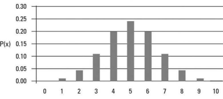
What is a probability distribution?
A probability distribution is a mathematical function that describes the likelihood of occurrence of different possible outcomes of a random variable. The probability of each possible outcome is represented by a range of values, called a probability distribution. Probability distributions are used to calculate the probability of various events, such as the likelihood of rolling a certain number on a dice. They can also be used to predict the probability of future events, such as the stock market. They are often represented using graphs, which makes it easy to visualize the probability of different outcomes. Probability distributions are important tools in statistics and are used in many different fields, from insurance to gambling. The picture below represents a sample of probability distribution.
There are two main types of probability distribution:
- Discrete probability distribution: A discrete probability distribution is a mathematical function that calculates the probability of discrete outcomes. In other words, it tells us how likely it is for something to happen given a certain number of events. It is the probability distribution of a discrete random variable. Discrete random variables can assume only discrete values (such as integers), whereas continuous random variables can assume any value that falls within a certain range. For example, if we flip a coin three times, there is a discrete probability distribution that calculates the probability of getting either three heads, two heads and one tail, or one head and two tails. A discrete probability distribution is often used when modeling events that have a finite number of outcomes and there is a known probability for each outcome. For example, rolling a die has only six possible outcomes and each outcome is equally likely, so we can model this event using a discrete probability distribution. Some other examples of discrete probability distributions include the binomial distribution and the Poisson distribution. The binomial distribution models the likelihood of success in a given number of independent trials, while the Poisson distribution models the likelihood of a given number of events occurring in a fixed period of time.
- Continuous probability distribution: A continuous probability distribution is a mathematical function that calculates the probability of continuous outcomes. In other words, it tells us how likely it is for something to happen given an infinite number of events. For example, if we flip a coin infinitely many times, there is a continuous probability distribution that calculates the probability of getting either all heads, all tails, or a mixture of both. Continuous distributions are often used to model quantities that can vary continuously, such as height, weight, or time. There are many examples of continuous probability distributions, including the normal distribution, the uniform distribution, and the exponential distribution. Each of these distributions has different applications and can be used to model different types of data. For instance, the normal distribution is often used to model data that are evenly distributed around a mean, such as test scores or heights. The uniform distribution is often used to model data that are equally likely to occur at any point within a specified interval, such as the length of time it takes for a light to turn on. The exponential distribution is often used to model data that occur at a constant rate, such as the time between arrivals of buses. In general, continuous distributions are defined by their probability density functions, which describe how the probabilities are distributed across the range of possible values.
How is probability used in machine learning?
Probability is used in machine learning to create models that can predict future events. Probability can help to determine how likely it is that a certain event will occur, and this information can be used to make predictions about future events. For example, if a machine learning model is trained on a data set of historical weather patterns, it can use probability to make predictions about the likelihood of future weather events. Probability is also used in machine learning to assess the accuracy of models. By testing a model on a data set and evaluating the results, the researcher can determine how likely it is that the model will accurately predict future events. Probability can therefore be used to improve the accuracy of machine learning models and make more accurate predictions about future events.
Probability is a fundamental tool in machine learning, used for making predictions and decisions based on data. In supervised learning, the probability is used to estimate the likelihood of each possible outcome, based on known features. This can be used for classification tasks, such as predicting whether an email is a spam or not. In unsupervised learning, the probability is used to find patterns in data, such as clusters of similar items. Probability is also used in reinforcement learning, where an agent learns by trial and error to take actions that maximize a reward.
Bayesian machine learning is a probabilistic approach to machine learning that is based on Bayesian probability theory. Bayesian probability is an approach to the probability that uses prior beliefs about the likelihood of certain events to update the probability after new evidence is observed. This can be used for both supervised and unsupervised learning tasks. For example, in supervised learning, a Bayesian model can be used to estimate the probability of each possible outcome, based on known features. This can be used for classification tasks, such as predicting whether an email is a spam or not. In unsupervised learning, a Bayesian model can be used to find patterns in data, such as clusters of similar items.
Bayesian machine learning is a powerful tool for making predictions and decisions based on data. It is based on sound probability theory and can be used for both supervised and unsupervised learning tasks. If you are working with machine learning, then you should definitely consider using Bayesian machine learning in your work.

Check out my books titled as Designing Decisions, and First Principles Thinking.
- The Watermelon Effect: When Green Metrics Lie - January 25, 2026
- Coefficient of Variation in Regression Modelling: Example - November 9, 2025
- Chunking Strategies for RAG with Examples - November 2, 2025

I found it very helpful. However the differences are not too understandable for me