In this post, you will learn about a feature selection technique called as Sequential Backward Selection using Python code example.
Feature selection is one of the key steps in training the most optimal model in order to achieve higher computational efficiency while training the model, and also reduce the the generalization error of the model by removing irrelevant features or noise. Some of the important feature selection techniques includes L-norm regularization and greedy search algorithms such as sequential forward or backward feature selection, especially for algorithms which don’t support regularization. It is of utmost importance for data scientists to learn these techniques in order to build optimal models.
Sequential backward selection algorithm aims to reduce the dimensionality of the initial feature subspace from N to K-features with a minimum reduction in the model performance to improve upon computational efficiency and reduce generalization error. The primary idea is to sequentially remove features from the given features list consisting of N features to reach to the list of K-features. At each stage of removal, the feature that causes the least performance loss gets removed. The search for features is based on combinatorial search algorithm where the subset of features get selected from combination and score is calculated for the subset and compared to other subsets. Note the usage of combinations class of itertools package in the code given below.
Here is the python code for sequential backward selection algorithm. The class takes the constructor as an instance of an estimator and subset of features to which the original feature space have to be reduced to. One can pass the training and test data set after feature scaling is done to determine the subset of features. The same is depicted in the python code given below.
The class provides a fit and transform method. Fit method determines the subset of features indices along with the accuracy scores. Pay attention to some of the following in the code:
- scores_ consists of best score with different number of dimensions
- subsets_ consists of feature indices representing features that led to best scores
from sklearn.metrics import accuracy_score
from itertools import combinations
from sklearn.base import clone
from numpy as np

class SequentialBackwardSearch():
    '''
    Instantiate with Estimator and given number of features
    '''
    def __init__(self, estimator, k_features):
        self.estimator = clone(estimator)
        self.k_features = k_features

    '''
    X_train - Training data Pandas dataframe
    X_test - Test data Pandas dataframe
    y_train - Training label Pandas dataframe
    y_test - Test data Pandas dataframe
    '''
    def fit(self, X_train, X_test, y_train, y_test):
        dim = X_train.shape[1]
        self.indices_ = tuple(range(dim))
        self.subsets_ = [self.indices_]
        score = self._calc_score(X_train.values, X_test.values,
                                 y_train.values, y_test.values, self.indices_)
        self.scores_ = [score]
        '''
        Iterate through all the dimensions until k_features is reached
        At the end of loop, dimension count is reduced by 1
        '''
        while dim > k_features:
            scores = []
            subsets = []
            '''
            Iterate through different combinations of features, train the model,
            record the score
            '''
            for p in combinations(self.indices_, r=dim - 1):
                score = self._calc_score(X_train.values, X_test.values, y_train.values, y_test.values, p)
                scores.append(score)
                subsets.append(p)
            #
            # Get the index of best score
            #
            best_score_index = np.argmax(scores)
            #
            # Record the best score
            #
            self.scores_.append(scores[best_score_index])
            #
            # Get the indices of features which gave best score
            #
            self.indices_ = subsets[best_score_index]
            #
            # Record the indices of features for best score
            #
            self.subsets_.append(self.indices_)
            dim -= 1 # Dimension is reduced by 1

    '''
    Transform training, test data set to the data set
    havng features which gave best score
    '''
    def transform(self, X):
        return X.values[:, self.indices_]

    '''
    Train models with specific set of features
    indices - indices of features
    '''
    def _calc_score(self, X_train, X_test, y_train, y_test, indices):
        self.estimator.fit(X_train[:, indices], y_train.ravel())
        y_pred = self.estimator.predict(X_test[:, indices])
        score = accuracy_score(y_test, y_pred)
        return score
Here is the python code representing how the instance of LogisticRegression (default solver = lbfgs) is used as an estimator. This is just for illustration purpose as one could apply L1 norm regularization technique with solver as liblinear for training the model with most appropriate features.
#
# Instantiate the estimator - LogisticRegression
#
lr = LogisticRegression(C=1.0, random_state=1)
#
# Number of features - 5
#
k_features = 5
#
# Instantiate SequentialBackwardSearch
#
sbs = SequentialBackwardSearch(lr, k_features)
#
# Fit the data to determine the k_features which give the
# most optimal model performance
#
sbs.fit(X_train, X_test, y_train, y_test)
#
# Transform the training data set to dataset having k_features
# giving most optimal model performance
#
X_train_kfeatures = sbs.transform(X_train)
#
# Transform the test data set to dataset having k_features
#
X_test_kfeatures = sbs.transform(X_test)
One could find the most optimal K-features using the following code:
X_train.columns[[sbs.indices_]] # sbs is an instance of SequentialBackwardSearch class
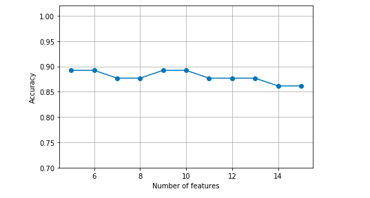
One could do the plot displaying most optimal features as each stage of reduction from N to K features vis-a-vis the model scores. Here is the python code:
k_features = [len(k) for k in sbs.subsets_]

from matplotlib.pyplot as plt

plt.plot(k_features, sbs.scores_, marker='o')
plt.ylim([0.7, 1.02])
plt.ylabel('Accuracy')
plt.xlabel('Number of features')
plt.grid()
plt.tight_layout()
plt.show()
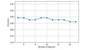
Here is how the plot would look like:

Some of the code snippets have been taken from Python Machine Learning book by Dr. Sebastian Raschka
- The Watermelon Effect: When Green Metrics Lie - January 25, 2026
- Coefficient of Variation in Regression Modelling: Example - November 9, 2025
- Chunking Strategies for RAG with Examples - November 2, 2025

I found it very helpful. However the differences are not too understandable for me