In this post, you will learn about how to train an optimal neural network using Learning Curves and Python Keras. As a data scientist, it is good to understand the concepts of learning curve vis-a-vis neural network classification model to select the most optimal configuration of neural network for training high-performance neural network.
In this post, the following topics have been covered:
- Concepts related to training a classification model using a neural network
- Python Keras code for creating the most optimal neural network using a learning curve
Training a Classification Neural Network Model using Keras
Here are some of the key aspects of training a neural network classification model using Keras:
- Determine whether it is a binary classification problem or multi-class classification problem
- For training any neural network using Keras, you may need to go through the following stages:
- Design & setup neural network architecture including a number of layers, number of nodes in each layer, and activation functions associated with each layer. One can use activation functions such as sigmoid, different variants of the such as ReLU, tanh, softmax function, etc. One can also try with different numbers of hidden layers having different numbers of nodes.
- Configure the neural network with optimizer function, loss function, and metrics
- Fit the neural network by setting up an optimal number of epochs and batch size.
- Preparing data for training the neural network model thereby creating training and test/validation data
- Use the learning curve to plot model accuracy and loss with respect to epochs and choose the most optimal value of hyperparameters including epochs size, batch size, neural network architecture configuration including layers and nodes configuration, activation functions, optimizer functions, loss function, etc.
Learning Curve of Neural Network Classification Model
Training a neural network requires deciding upon the optimal number of layers, nodes, and activation functions. In addition, it is also important to select the most optimal values of epochs and batch size which will be used to fit a neural network model. This is where the learning curve comes into the picture.
The learning curve represents the neural network model accuracy and loss plots with respect to training and validation data set after each epoch of training are run. The learning curve helps in determining the optimal value of hyperparameters for creating the most optimal neural network in order to avoid overfitting and help achieve greater generalization in making correct predictions on unseen data (population).
In this section, a binary classification model is trained based on a neural network using the Sklearn breast cancer dataset. The data used in this post is pretty small. Ideally, neural network models require a large volume of data for training purposes in order to achieve higher model performance. Pay attention to some of the following aspects showcased in the Python Keras code given below:
- Loading Sklearn breast cancer dataset
- Setting up the neural network instance; A sequential network instance is created.
- Configure the neural network with layers, number of nodes in each layer, and associated activation functions. There are two hidden layers having 32 nodes each is created with activation function as ‘relu’
- Create training and test data split
- Fit the neural network; Network is fit with epoch size as 4 and batch size as 20.
import numpy as np
from sklearn import datasets
from sklearn.model_selection import train_test_split
from keras import models
from keras import layers
from keras import optimizers
#
# Load Sklearn Breast Cancer Dataset
#
bc = datasets.load_breast_cancer()
X = bc.data
y = bc.target
#
# Set up the network
#
network = models.Sequential()
network.add(layers.Dense(32, activation='relu', input_shape=(30,)))
network.add(layers.Dense(32, activation='relu'))
network.add(layers.Dense(1, activation='sigmoid'))
#
# Configure the network with optimizer, loss function and accuracy
#
network.compile(optimizer=optimizers.RMSprop(lr=0.01),
                loss='binary_crossentropy',
                metrics=['accuracy'])
#
# Create training and test split
#
X_train, X_test, y_train, y_test = train_test_split(X, y, test_size=0.3, stratify=y, random_state=42)
#
# Fit the network
#
history = network.fit(X_train, y_train,
                    validation_data=(X_test, y_test),
                    epochs=4,
                    batch_size=20)
Here is the Python Keras code for plotting the learning curve plotting model accuracy vs epochs. There are two different plots given below:
import matplotlib.pyplot as plt

history_dict = history.history
loss_values = history_dict['loss']
val_loss_values = history_dict['val_loss']
accuracy = history_dict['accuracy']
val_accuracy = history_dict['val_accuracy']

epochs = range(1, len(loss_values) + 1)
fig, ax = plt.subplots(1, 2, figsize=(14, 6))
#
# Plot the model accuracy vs Epochs
#
ax[0].plot(epochs, accuracy, 'bo', label='Training accuracy')
ax[0].plot(epochs, val_accuracy, 'b', label='Validation accuracy')
ax[0].set_title('Training & Validation Accuracy', fontsize=16)
ax[0].set_xlabel('Epochs', fontsize=16)
ax[0].set_ylabel('Accuracy', fontsize=16)
ax[0].legend()
#
# Plot the loss vs Epochs
#
ax[1].plot(epochs, loss_values, 'bo', label='Training loss')
ax[1].plot(epochs, val_loss_values, 'b', label='Validation loss')
ax[1].set_title('Training & Validation Loss', fontsize=16)
ax[1].set_xlabel('Epochs', fontsize=16)
ax[1].set_ylabel('Loss', fontsize=16)
ax[1].legend()
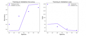
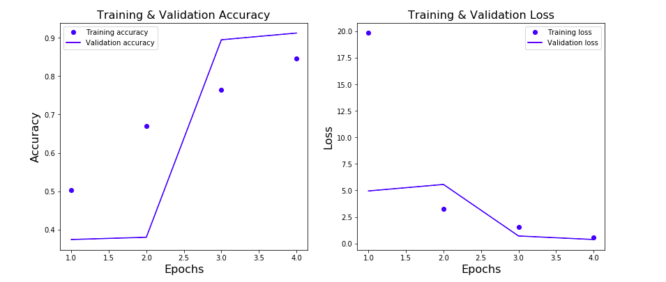
Executing the above code will result in the following plot. Pay attention to some of the following in the plot given below:
- In accuracy vs epochs plot, note that validation accuracy at epoch value 4 is higher than the model accuracy with the training data
- In loss vs epochs plot, note that the loss with both training and validation at epoch value = 4 is low.
Conclusions
Here is the summary of what got covered in relation to using learning curve to select most appropriate configuration for neural network architecture for training a classification model:
- Learning curve is used to plot the model training / validation accuracy and training / validation loss vs epochs.
- Epochs where validation accuracy is lesser than training accuracy represents the overfitting
- Epochs where validation loss is greater than than training loss represents overfitting
- What can be configured for neural network classification model are – 1. Number of layers 2. Number of nodes in each layer 3. Activation functions in each node 4. Optimizer function 5. Loss function 6. Metrics

Check out my latest book titled as First Principles Thinking: Building winning products using first principles thinking.
- Mathematics Topics for Machine Learning Beginners - July 6, 2025
- Questions to Ask When Thinking Like a Product Leader - July 3, 2025
- Three Approaches to Creating AI Agents: Code Examples - June 27, 2025
I found it very helpful. However the differences are not too understandable for me