In this post, you will learn about how to calculate Eigenvalues and Eigenvectors using Python code examples. Before getting ahead and learning the code examples, you may want to check out this post on when & why to use Eigenvalues and Eigenvectors. As a machine learning Engineer / Data Scientist, you must get a good understanding of Eigenvalues / Eigenvectors concepts as it proves to be very useful in feature extraction techniques such as principal components analysis. Python Numpy package is used for illustration purpose. The following topics are covered in this post:
- Creating Eigenvectors / Eigenvalues using Numpy Linalg module
- Re-creating original transformation matrix from eigenvalues & eigenvectors
Creating Eigenvectors / Eigenvalues using Numpy
In this section, you will learn about how to create Eigenvalues and Eigenvectors for a given square matrix (transformation matrix) using Python Numpy library. Here are the steps:
- Create a sample Numpy array representing a set of dummy independent variables / features
- Scale the features
- Calculate the n x n covariance matrix. Note that the transpose of the matrix is taken. One can use np.cov(students_scaled, rowvar=False) instead to represent that columns represent the variables.
- Calculate the eigenvalues and eigenvectors using Numpy linalg.eig method. This method is designed to operate on both symmetric and non-symmetric square matrices. There is another method such as linalg.eigh which is used to decompose Hermitian matrices which is nothing but a complex square matrix that is equal to its own conjugate transpose. The linalg.eigh method is considered to be numerically more stable approach to working with symmetric matrices such as the covariance matrix.
import numpy as np
from sklearn.preprocessing import StandardScaler
from numpy.linalg import eig
#
# Percentage of marks and no. of hours studied
#
students = np.array([[85.4, 5],
            [82.3, 6],
            [97, 7],
            [96.5, 6.5]])
#
# Scale the features
#
sc = StandardScaler()
students_scaled = sc.fit_transform(students)
#
# Calculate covariance matrix; One can also use the following
# code: np.cov(students_scaled, rowvar=False)
#
cov_matrix = np.cov(students_scaled.T)
#
# Calculate Eigenvalues and Eigenmatrix
#
eigenvalues, eigenvectors = eig(cov_matrix)
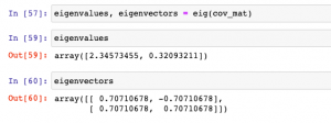
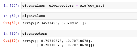
Here is how the output of above looks like:

Let’s confirm whether the above is correct by calculating LHS and RHS of the following and making sure that LHS = RHS. A represents the transformation matrix (cob_matrix in above example), x represents eigenvectors and [latex]\lambda[/latex] represents eigenvalues
[latex]
Ax = \lambda x
[/latex]
Here is the code comparing LHS to RHS
#
# LHS
#
cov_matrix.dot(eigenvectors[:, 0])
#
# RHS
#
eigenvalues[0]*eigenvectors[:, 0]
From the output represented in the picture below, it does confirm that above calculation done by Numpy linalg.eig method is correct.

Conclusion
Here is what you learned in this post:
- One will require to scale the data before calculating its Eigenvalues and Eigenvectors
- One will need to have the transformation matrix as square matrix N x N representing N dimensions in order to calculate N eigenvalues and Eigenvectors
- Numpy linear algebra module linalg can be used along with eig to determine Eigenvalues and Eigenvectors.
- The Watermelon Effect: When Green Metrics Lie - January 25, 2026
- Coefficient of Variation in Regression Modelling: Example - November 9, 2025
- Chunking Strategies for RAG with Examples - November 2, 2025

VERY USEFUL
Thank you