Forecasting is the process of predicting future events based on past and present data. Time-series forecasting is a type of forecasting that predicts future events based on time-stamped data points. Time-series forecasting models are an essential tool for any organization or individual who wants to make informed decisions based on future events or trends. From stock market predictions to weather forecasting, time-series models help us to understand and forecast changes over time. However, with so many different types of models available, it can be challenging to determine which one is best suited for a particular scenario.
There are many different types of time-series forecasting models, each with its own strengths and weaknesses. Understanding the differences between these models is crucial for anyone looking to use most appropriate modeling technique for the time-series data. In this blog post, we will discuss the most common time-series forecasting machine learning models such as the following, and provide examples of how they can be used to predict future events.
- Autoregressive (AR) model
- Moving average (MA) model
- Autoregressive moving average (ARMA) model
- Autoregressive integrated moving average (ARIMA) model
- Seasonal autoregressive integrated moving average (SARIMA) model
- Vector autoregressive (VAR) model
- Vector error correction (VECM) model
Before we get ahead, lets quickly learn about what is time-series forecasting?
What are time-series forecasting models?
Time-series forecasting is the process of using past data to predict future events. Time-series forecasting models are statistical models used to make predictions about future values based on historical data points arranged in chronological order. These models analyze trends and patterns in the data and extrapolate them to make predictions about future values. These models are commonly used in business and finance to predict sales or stock prices, and in science to predict weather patterns. Time-series forecasting models is a special class of predictive modeling that is used to forecast future events.
How are time series forecasting models different from other predictive modeling techniques?
Time-series forecasting models are different from other predictive modeling techniques in various different manner such as the following:
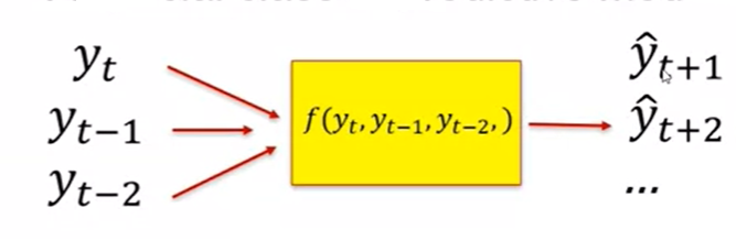
- Time-series models rely on historical data that is arranged in chronological order, whereas other models may use cross-sectional data or other non-time-related variables. The response variable to be forecasted is continuous in nature while input data are past values of variable of interest (response variable). The following picture represents the same. The variable to be predicted and the input variable are one and the same. [latex]Y_t, Y_{t-1}, Y_{t-2}[/latex] are values of the past and [latex]Y_{t+1}, Y_{t+2}[/latex] are values in future which are to be predicted.
- Time-series models account for the temporal dependencies between data points, whereas other models assume that each data point is independent of the others.
- Time-series models often use specialized algorithms and techniques, such as ARIMA or exponential smoothing, which are designed specifically for time-series data.
What are different characteristics of a time-series data?
There are several characteristic of a time-series data that need to be taken into account when modeling time-series data.
- Time dependence: Time-series data is collected over time, with each observation representing a data point at a specific point in time. As a result, time-series data exhibits temporal dependence, meaning that each data point is influenced by the previous ones.
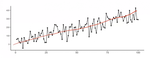
- Trend: The most important one is the trend of the data. Time-series data often exhibit a trend, which is a gradual increase or decrease in the value of the data over time. The trend needs to be accounted for in the time-series forecasting model. The picture below shows an upward trend in the time-series data.
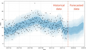
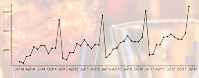
- Seasonality: Another important characteristic of time-series data is the seasonal effect. Seasonal effects are patterns that occur regularly (yearly, quarterly, monthly, etc) in the data due to seasonal factors such as holidays or changes in weather. The seasonal effect needs to be accounted for in the forecasting model. The picture below shows the seasonality in the data:
- Noise: The final characteristic of time-series data is the random error. Random error is noise that is present in the data and affects the accuracy of the forecast. The random error needs to be accounted for in the forecasting model.


Different classes of time-series data
There are two different classes of time-series data: stationary and non-stationary data.
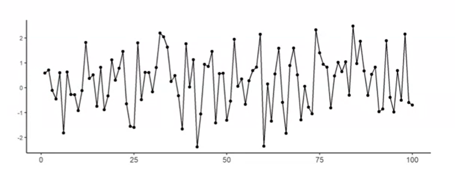
- Stationary time-series data is one where the statistical properties of the data do not change over time. In other words, the data does not exhibit any trend, seasonality, or other patterns that would cause these statistical properties to change. The random error is the only source of variability in the data set. For example, the number of people visiting a library on a random weekday can be called stationary data, which does not show any significant trend or seasonality. Or, the daily closing price of a stable blue-chip stock that has no significant trend or seasonality can also be termed as stationary data. The picture below represents time-series stationary data with no sign of trends or seasonality.

- Non-stationary time-series data is a time-series data set that exhibits a trend or a seasonal effect. The random error is no longer the only source of variability in the data set. Non-stationary time-series data requires additional pre-processing, such as detrending or differencing, to remove the non-stationarity before modeling and forecasting can be done accurately. The following are some examples of non-stationary time-series data:
- The annual sales figures of a company that has been growing steadily over the years, showing a clear trend.
- The monthly temperature readings of a city, which exhibit a seasonal pattern as temperatures rise and fall with the seasons.
- The stock prices of a new startup that has experienced significant growth in a short period, showing an upward trend over time.
Autoregressive (AR) model
Autoregressive (AR) models are defined as regression models in which the dependent or response variable is a linear function of past values of the dependent/response variable. The order of an autoregressive model is denoted as ‘p’, which represents the number of lags used to predict the current value. For example, if p=0, then it means that we are predicting the current time-step (t) based on the previous time-step (t-0). If p=n, then we are predicting time-step (t) based on n past time-steps.
The general form of an autoregressive model can be represented as:
[latex]Y_t = c + \phi_p Y_{t-p} + \varepsilon_t[/latex]
Moving average (MA) model
A moving average (MA) is a type of model used for time-series forecasting. The moving average models are primarily used for stationary data, the data where we don’t see significant trends or seasonality. There are two different kinds of moving average model. They are simple moving average and weighted moving average model.
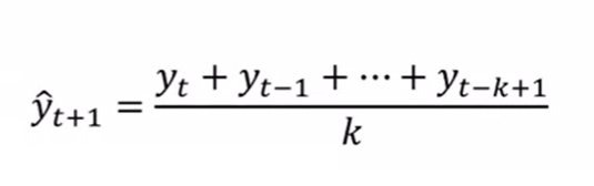
- A Simple Moving Average (SMA) is a type of moving Average model that uses a fixed number of data points for the averaging calculation. This type of MA is often used for time-series forecasting, because it is easy to calculate and can be implemented in a variety of programming languages. Here is a great video on simple moving average model and how could you calculate performance metrics such as MAE / MAD and MSE / RMSE. The following is the formula for simple moving average model. Larger value of K results in smoother forecast models.
- A Weighted Moving Average (WMA) is a type of moving Average model that uses a weighting scheme to give more importance to more recent data points. This type of MA can be used for time-series forecasting, and can help to reduce the impact of older data points on the average. Here is a great video on weighted moving average model and how could you calculate performance metrics such as MAE / MAD and MSE / RMSE.
One real-world use case for Moving Average model is stock market analysis. Moving average models can be used to help predict future stock prices by taking into account past prices. Another real-world use case is time-series forecasting of sales data. Moving average models can be used to help forecast future sales by taking into account past sales data.
There are a few factors to consider when deciding whether to use a simple or weighted Moving Average model. One factor is the type of data that is being averaged. If the data is stationary (doesn’t have any trends or seasonality), then a simple Moving Average model can be used. If the data has significant trends or seasonality, then a weighted Moving Average model should be used. Another factor to consider is how much weight to give to each data point. If more recent data points are more important, then a weighted Moving Average model should be used.
Autoregressive moving average (ARMA) model
The autoregressive moving average (ARMA) model is a combination of the autoregressive and moving average models. The ARMA model is defined as a regression model in which the dependent/response variable is a linear function of past values of both the dependent/response variable and the error term. The order of an ARMA model is represented by ‘p’ for the autoregressive part and ‘q’ for the moving average part. For example, if p=0 and q=0, then it means that we are predicting time-step (t) based on time-step (t) only. If p=n and q=m, then we are predicting time-step (t) based on n past time-steps of the dependent/response variable and m past time-steps of the error term.
The general form of an ARMA model can be represented as:
[latex]Y_t = c + \phi_p Y_{t-p} + \theta_q \varepsilon_{t-q} + \varepsilon_t[/latex]
Autoregressive integrated moving average (ARIMA) model
The autoregressive integrated moving average (ARIMA) model is a generalization of the ARMA model. The ARIMA model is defined as a regression model in which the dependent/response variable is a linear function of past values of both the dependent/response variable and the error term, where the error term has been differentiated ‘d’ times. The order of an ARIMA model is represented by ‘p’ for the autoregressive part, ‘q’ for the moving average part, and ‘d’ for the differencing part. For example, if p=0, q=0, and d=0, then it means that we are predicting time-step (t) based on time-step (t) only. If p=n, q=m, and d=k, then we are predicting time-step (t) based on n past time-steps of the dependent/response variable, m past time-steps of the error term, and k past time-steps of the differenced error term.
The general form of an ARIMA model can be represented as:
[latex]Y_t = c + \phi_p Y_{t-p} + \theta_q \varepsilon_{t-q} + \delta^d Y_t[/latex]
The interpretation of autoregressive integrated moving average (ARIMA) models is similar to that of autoregressive moving average (ARMA) models. The main difference between ARIMA and ARMA models is that ARIMA models can be used to model time-series data that is non-stationary, whereas ARMA models can only be used to model time-series data that is stationary.
Seasonal autoregressive integrated moving average (SARIMA) model
SARIMA is a type of time-series forecasting model that takes into account both seasonality and autocorrelation. SARIMA models are based on a combination of differencing, autoregression, and moving average processes. These models can be used to forecast short-term or long-term trends in data. SARIMA models are generally considered to be more accurate than other types of time-series forecasting models, such as ARIMA models. SARIMA models are also relatively easy to interpret and use.
The SARIMA model can be used to forecast demand for a product or service over the course of a year. The model takes into account sales data from previous years as well as seasonality (e.g., holiday sales). SARIMA can also be used to forecast other time-series data, such as stock prices or weather patterns. The SARIMA model is a generalization of the ARIMA model (which only accounts for autocorrelation), and it can be used to forecast data with seasonality.
Vector autoregressive (VAR) model
The vector autoregressive (VAR) model can be defined as a multivariate time-series model that captures the linear interdependence among multiple time-series variables. In addition to the dependent variables, the VAR model also includes one or more lagged values of each dependent variable as independent variables. Example: A VAR(p) for a bivariate time-series [latex]{y_t,x_t}[/latex] would be
[latex]y_t = c + A_iy_{t-i} + A_jx_{t-j} + u_t[/latex]
where p is the lag order, c is a vector of constants, A_i and A_j are matrices of coefficients, and u_t is white noise.
The above equation can be rewritten in vector form as
[latex]Y_t = c + A_0Y_{t-0} + A_pY_{t-p} + u_t[/latex]
where Y_t is a vector consisting of the time-series variables y_t and x_t, c is a vector of constants, A_0 is a matrix of coefficients, and u_t is white noise.
The VAR model can be estimated using ordinary least squares (OLS). Once the model has been estimated, it can be used to make forecasts. For example, if we wanted to forecast the value of y at time t+h, we would use the following equation:
[latex]y_{t+h} = c + A_iy_{t+h-i} + A_jx_{t+h-j}[/latex]
where h is the forecasting horizon.
The VAR model is a generalization of the univariate autoregressive (AR) model and the multivariate linear regression model. It can be used to study the dynamics of a single time-series variable or multiple time-series variables. One advantage of the VAR model is that it can be easily estimated using OLS. Another advantage is that it can be used to make forecasts. One disadvantage of the VAR model is that it can be difficult to interpret. For example, it can be hard to determine which time-series variables are influencing each other.
Vector Error Correction Model (VECM)
The Vector Error Correction Model (VECM) is a type of time-series model that is often used for forecasting economic data. VECM is an extension of the traditional vector autoregression (VAR) model. VECM was first introduced by Engle and Granger (1987). VECM models are similar to VAR models, but they incorporate a “correction” term that accounts for the fact that errors in one period are likely to be corrected in subsequent periods. This makes VECM models more accurate than VAR models when forecasting data with significant serial correlation. VECM models are also relatively easy to interpret since the coefficients can be directly interpreted as the impact of one variable on another. VECM has become a popular tool in econometrics and finance due to its flexibility and ease of use.
The VECM has several advantages over the VAR model. First, it is easier to interpret the results of a VECM than a VAR. Second, the VECM can be used to test for co-integration among time series variables, while the VAR cannot. Finally, the VECM can be applied to non-stationary time series data, while the VAR cannot.
The disadvantages of the VECM include its complexity and the fact that it requires a large amount of data to produce reliable results. In addition, the VECM is sensitive to outliers and changes in the time-series data.
Time-series forecasting models are used to predict future values of time-series data. In this blog post, we discussed different types of time-series forecasting models such as AR, MA, ARMA, ARIMA, the SARIMA model, the vector autoregressive (VAR) model, and the vector error correction model (VECM). All of these models have their own advantages and disadvantages. Choose the time-series forecasting model that is best suited for your data and your forecasting needs.

Check out my latest book titled as First Principles Thinking: Building winning products using first principles thinking.
- Mathematics Topics for Machine Learning Beginners - July 6, 2025
- Questions to Ask When Thinking Like a Product Leader - July 3, 2025
- Three Approaches to Creating AI Agents: Code Examples - June 27, 2025
Good evening Kumar,
I am an MSc student is IT Project Management and want to do my project on Forecasting the impact of project management methodologies on software projects which is a new area from my systematic review.
please what kind of time series will be suitable for this research.
I will want to consider time as the variable.
Please i am open to suggestion.
Thank you.
Hi, Project management methodologies can impact software projects at different levels, such as project duration, cost, quality, and customer satisfaction. Hence, the choice of the time series should depend on the specific aspect of the impact that the research aims to forecast.
Given we are are looking at univariate time series model, some common types of time series models that can be used for forecasting include ARMA, ARIMA, Prophet, LSTM, etc. The choice of the model should depend on the nature of the data, the research question, and the available computing resources.
The time series data should be analyzed to identify its characteristics such as trend, seasonality, cyclicality, and other patterns. If the data is stationary, then models such as ARMA or Prophet may be more appropriate. If the data is non-stationary, then models that can handle non-stationary data, such as ARIMA or LSTM, may be more suitable. There are other factors such as time horizon, data complexity, etc which are deciding factors for which type of time series forecasting should we opt for?