In this post, you will learn about how to train a decision tree classifier machine learning model using Python. The following points will be covered in this post:
- What is decision tree?
- Decision tree python code sample
What is Decision Tree?
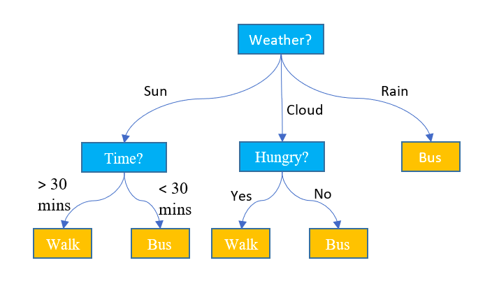
Simply speaking, the decision tree algorithm breaks the data points into decision nodes resulting in a tree structure. The decision nodes represent the question based on which the data is split further into two or more child nodes. The tree is created until the data points at a specific child node is pure (all data belongs to one class). The criteria for creating the most optimal decision questions is the information gain. The diagram below represents a sample decision tree.

Training a machine learning model using a decision tree classification algorithm is about finding the decision tree boundaries.
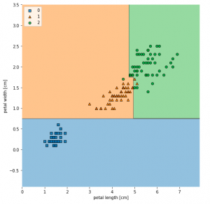
Decision trees build complex decision boundaries by dividing the feature space into rectangles. Here is a sample of how decision boundaries look like after model trained using a decision tree algorithm classifies the Sklearn IRIS data points. The feature space consists of two features namely petal length and petal width. The code sample is given later below.

Decision Tree Python Code Sample
Here is the code sample which can be used to train a decision tree classifier.
import pandas as pd
import numpy as np
import matplotlib.pyplot as plt
from sklearn import datasets
from sklearn.model_selection import train_test_split
from sklearn.tree import DecisionTreeClassifier

iris = datasets.load_iris()
X = iris.data[:, 2:]
y = iris.target

X_train, X_test, y_train, y_test = train_test_split(X, y, test_size=0.3, random_state=1, stratify=y)

clf_tree = DecisionTreeClassifier(criterion='gini', max_depth=4, random_state=1)
clf_tree.fit(X_train, y_train)
Visualizing Decision Tree Model Decision Boundaries
Here is the code which can be used to create the decision tree boundaries shown in fig 2. Note that the package mlxtend is used for creating decision tree boundaries.
from mlxtend.plotting import plot_decision_regions

X_combined = np.vstack((X_train, X_test))
y_combined = np.hstack((y_train, y_test))

fig, ax = plt.subplots(figsize=(7, 7))
plot_decision_regions(X_combined, y_combined, clf=clf_tree)
plt.xlabel('petal length [cm]')
plt.ylabel('petal width [cm]')
plt.legend(loc='upper left')
plt.tight_layout()
plt.show()
Visualizing Decision Tree in the Tree Structure
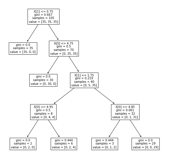
Here is the code which can be used visualize the tree structure created as part of training the model. plot_tree function from sklearn tree class is used to create the tree structure. Here is the code:
from sklearn import tree

fig, ax = plt.subplots(figsize=(10, 10))
tree.plot_tree(clf_tree, fontsize=10)
plt.show()
Here is how the tree would look after the tree is drawn using the above command. Note the usage of plt.subplots(figsize=(10, 10)) for creating a larger diagram of the tree. Otherwise, the tree created is very small.

In the follow-up article, you will learn about how to draw nicer visualizations of decision tree using graphviz package. Also, you will learn some key concepts in relation to decision tree classifier such as information gain (entropy, gini etc).
- The Watermelon Effect: When Green Metrics Lie - January 25, 2026
- Coefficient of Variation in Regression Modelling: Example - November 9, 2025
- Chunking Strategies for RAG with Examples - November 2, 2025

I found it very helpful. However the differences are not too understandable for me