In this post, you will learn about concepts of neural networks with the help of mathematical models examples. In simple words, you will learn about how to represent the neural networks using mathematical equations. As a data scientist / machine learning researcher, it would be good to get a sense of how the neural networks can be converted into a bunch of mathematical equations for calculating different values. Having a good understanding of representing the activation function output of different computation units / nodes / neuron in different layers would help in understanding back propagation algorithm in a better and easier manner. This will be dealt in one of the future posts.
Single Layer Neural Network (Perceptron)
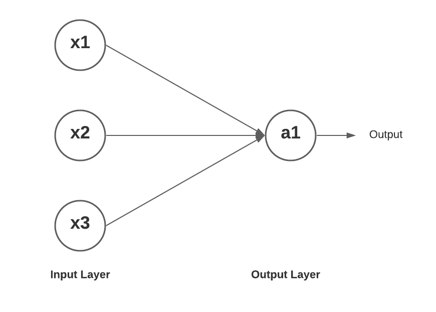
Here is how a single layer neural network looks like. You may want to check out my post on Perceptron – Perceptron explained with Python example.

Here is how the mathematical equation would look like for getting the value of a1 (output node) as a function of input x1, x2, x3.
[latex]a^{(2)}_1 = g(\theta^{(1)}_{10}x_0 + \theta^{(1)}_{11}x_1 + \theta^{(1)}_{12}x_2 + \theta^{(1)}_{13}x_3)[/latex]
.
In the above equation, the superscript of weight represents the layer and the subscript of weights represent the weight of connection between the input node to output node. Thus, [latex]\theta^{(1)}_12[/latex] represents the weight of the first layer between the node 1 in next layer and node 2 in current layer.
Neural Network with One Hidden Layer
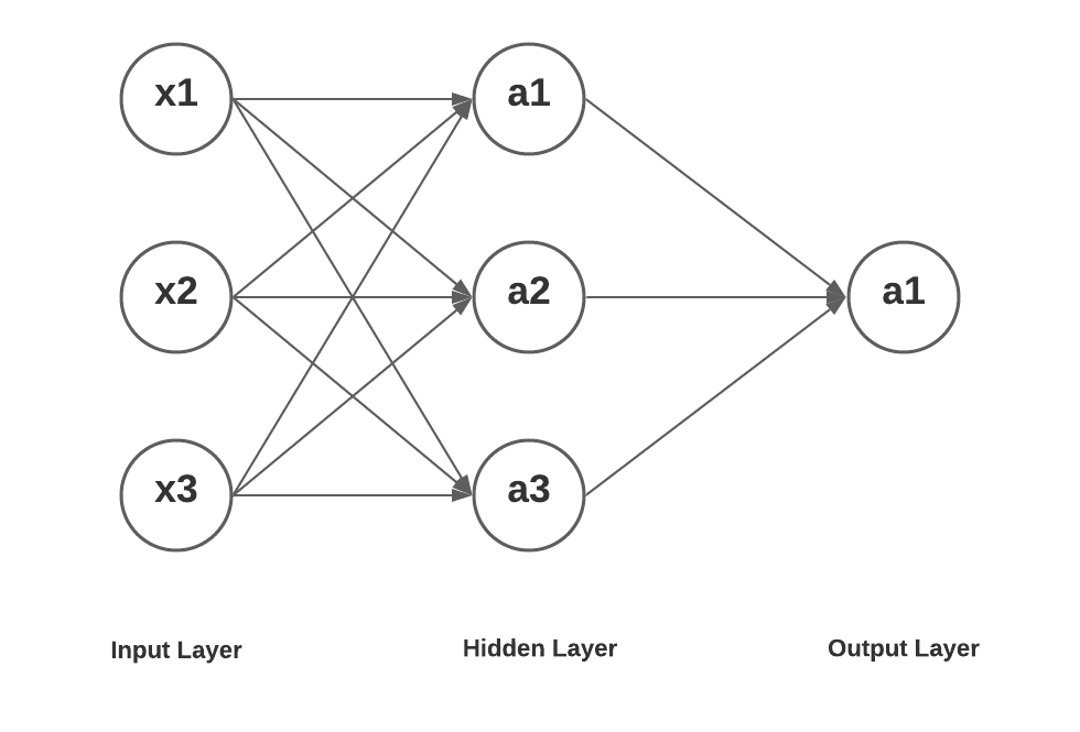
Here is a neural network with one hidden layer having three units, an input layer with 3 input units and an output layer with one unit.

Here is how the mathematical equation would look like for getting the value of a1, a2 and a3 in layer 2 as a function of input x1, x2, x3. Further, the value of a1 in layer 3 is represented as a function of value of a1, a2 and a3 in layer 2.
As a first step, lets represent the output values processed in three hidden units in the hidden layer. Input layer is represented as layer 1, hidden layer as layer 2 and output layer as layer 3.
[latex]a^{(2)}_1 = g(\theta^{(1)}_{10}x_0 + \theta^{(1)}_{11}x_1 + \theta^{(1)}_{12}x_2 + \theta^{(1)}_{13}x_3)[/latex]
.
[latex]a^{(2)}_2 = g(\theta^{(1)}_{20}x_0 + \theta^{(1)}_{21}x_1 + \theta^{(1)}_{22}x_2 + \theta^{(1)}_{23}x_3)[/latex]
.
[latex]a^{(2)}_3= g(\theta^{(1)}_{30}x_0 + \theta^{(1)}_{31}x_1 + \theta^{(1)}_{32}x_2 + \theta^{(1)}_{33}x_3)[/latex]
.
Lets determine the output value of node / unit in the output layer. The value gets represented as a function of a1, a2 and a3 in the previous nodes / units which could be represented as value of x1, x2 and x3 in the input layer.
[latex]a^{(3)}_1 = g(\theta^{(2)}_{10}a^{(2)}_0 + \theta^{(2)}_{11}a^{(2)}_1 + \theta^{(2)}_{12}a^{(2)}_2 + \theta^{(2)}_{13}a^{(2)}_3)[/latex]
.
Neural Network with One Hidden Layer (3 units) and Output Layer (2 units)
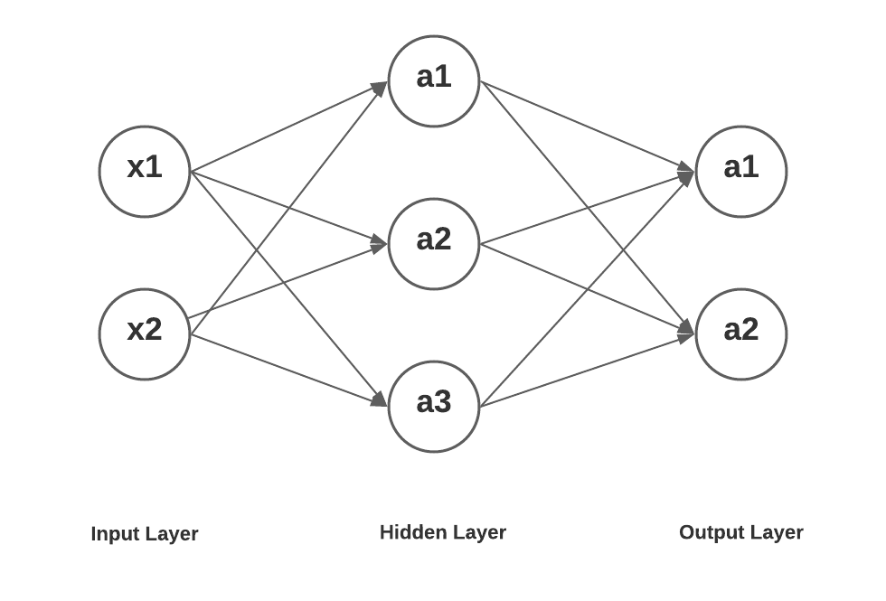
Here is a neural network with one hidden layer having three units, an input layer with 2 input units and an output layer with 2 units.

Here is how the mathematical equation would look like for getting the value of a1, a2 and a3 in layer 2 as a function of input x1, x2. Further, the value of a1 and a2 in layer 3 is represented as a function of value of a1, a2 and a3 in layer 2.
As a first step, lets represent the output values processed in three hidden units in the hidden layer. Input layer is represented as layer 1, hidden layer as layer 2 and output layer as layer 3.
[latex]a^{(2)}_1 = g(\theta^{(1)}_{10}x_0 + \theta^{(1)}_{11}x_1 + \theta^{(1)}_{12}x_2)[/latex]
.
[latex]a^{(2)}_2 = g(\theta^{(1)}_{20}x_0 + \theta^{(1)}_{21}x_1 + \theta^{(1)}_{22}x_2)[/latex]
.
[latex]a^{(2)}_3= g(\theta^{(1)}_{30}x_0 + \theta^{(1)}_{31}x_1 + \theta^{(1)}_{32}x_2)[/latex]
.
Let’s determine the output value of nodes / units in the output layer. The value gets represented as a function of a1, a2 and a3 in the previous nodes / units which could be represented as value of x1, x2 and x3 in the input layer.
[latex]a^{(3)}_1 = g(\theta^{(2)}_{10}a^{(2)}_0 + \theta^{(2)}_{11}a^{(2)}_1 + \theta^{(2)}_{12}a^{(2)}_2 + \theta^{(2)}_{13}a^{(2)}_3)[/latex]
.
[latex]a^{(3)}_2 = g(\theta^{(2)}_{20}a^{(2)}_0 + \theta^{(2)}_{21}a^{(2)}_1 + \theta^{(2)}_{22}a^{(2)}_2 + \theta^{(2)}_{23}a^{(2)}_3)[/latex]
.
Deep Learning Networks with 2 Hidden Layers
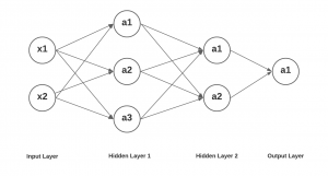
Lastly, let’s take a look at how the output values of nodes / unit a1 in output layer can be expressed as mathematical computations as a function of input signals x1 and x2. Here is the diagram of the deep learning network having two hidden layers, one having three nodes / units and other having 2 nodes / units Then there is an input layer having two input nodes and an output layer having one output node / unit. Here is the diagram of a simplistic deep learning network.

The values at layer 2 (a1, a2 and a3) and layer 3 (a1 and a2) will remain same as shown in the previous section. Lets represent the value of 1 in the output layer as a function of values of a1 and a2 in the previous layer (layer 3).
[latex]a^{(4)}_1 = g(\theta^{(3)}_{10}a^{(3)}_0 + \theta^{(3)}_{11}a^{(3)}_1 + \theta^{(3)}_{12}a^{(3)}_2)[/latex]
.
Conclusions
Here is the summary of what you learned in this post regarding representing neural networks as mathematical models:
- It is important to understand the notations in which you will represent neural network as mathematical models / equations
- First layer / input layer is assigned layer 1, hidden layer is assigned layer 2 and output layer is assigned layer 3.
- Weights between input node in one layer to the node in next layer is assigned superscript, the number, which is value of the layer consisting of input node. The subscript of weight consists of two numbers – number representing node in next layer followed by number of input node.
- The Watermelon Effect: When Green Metrics Lie - January 25, 2026
- Coefficient of Variation in Regression Modelling: Example - November 9, 2025
- Chunking Strategies for RAG with Examples - November 2, 2025

I found it very helpful. However the differences are not too understandable for me