Optimization problems containing many local minima remains a critical problem in a variety of domains, including operations research, informatics, and material design. Efficient global optimization remains a problem of general research interest, with applications to a range of fields including operations design, network analysis, and bioinformatics. Within the fields of chemical physics and material design, efficient global optimization is particularly important for finding low potential energy configurations of isolated groups of atoms (clusters) and periodic systems (crystals). In case of Machine learning (ML) algorithms, theer is a need for optimising (minimising) the cost or loss function. In order to become very good at finding solutions to optimisation problems (relating to minimising functions) including machine learning based problems, one must get a good understanding of the concepts of Local minima / global minima and local maxima / global maxima. In this post, you will learning about local minima and global minima.
Local Minima and Global Minima
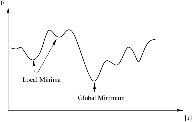
The point at which a function takes the minimum value is called global minima. However, when the goal is to minimize the function and solved using optimization algorithms such as gradient descent, it may so happen that function may appear to have a minimum value at different points. Those several points which appear to be minima but are not the point where the function actually takes the minimum value are called local minima. Machine learning algorithms such as gradient descent algorithms may get stuck in local minima during the training of the models. Gradient descent is able to find local minima most of the time and not global minima because the gradient does not point in the direction of the steepest descent. Current techniques to find global minima either require extremely high iteration counts or a large number of random restarts for good performance. Global optimization problems can also be quite difficult when high loss barriers exist between local minima.
Take a look at the following picture to understand the concept of local minima and global minima.

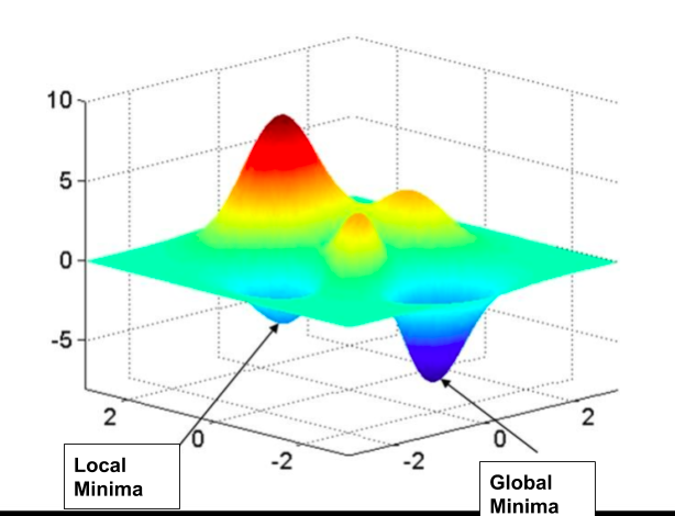
When you draw the function in 3-dimensional space, this is how the local minima and global minima will look like:

In order to find whether a point is local minima or global minima, one would need to find all possible minima of the function.
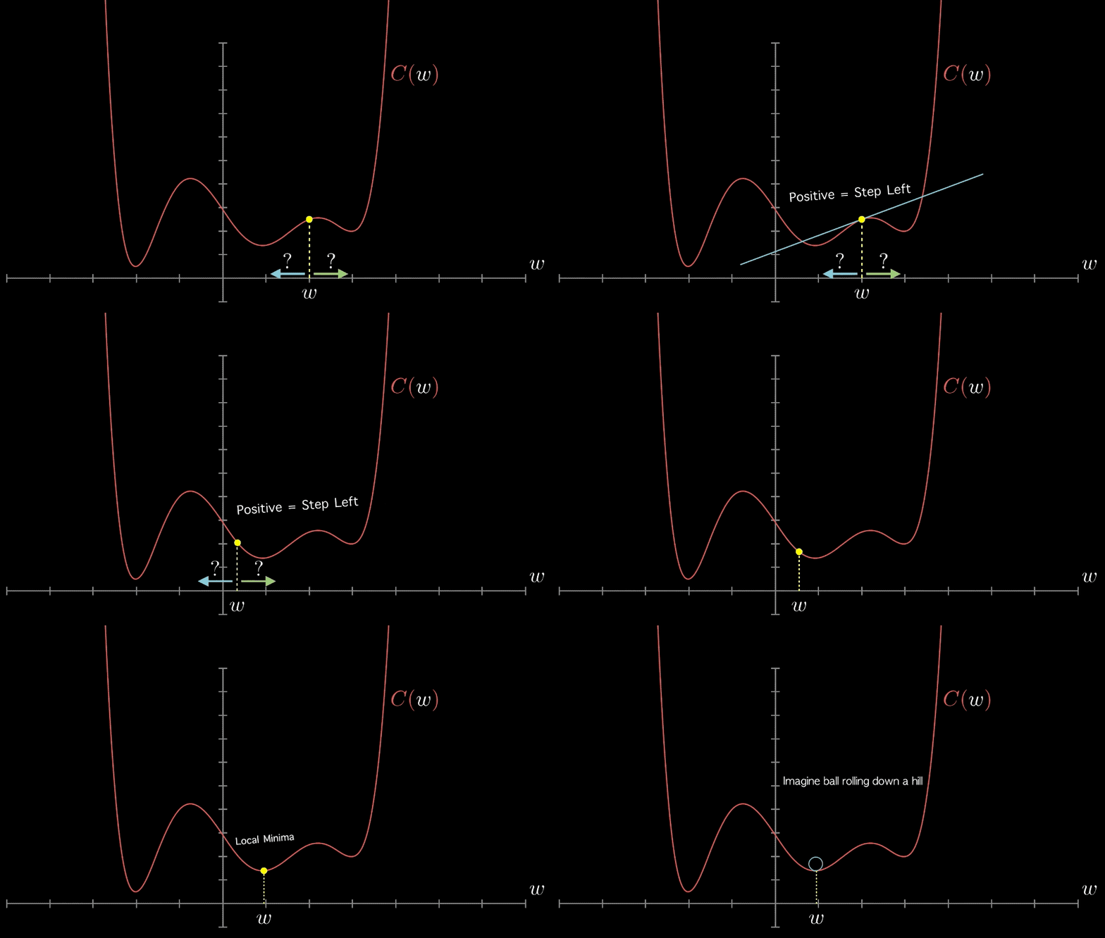
Here is an animation that can help you understand the difference between local and global minima in a better manner.

Pay attention to some of the following in the above animation:
- The gradient at different points is found out.
- If the gradient value is positive at a point, it will be required to move to left or reduce the weight.
- If the gradient value is negative at a point, it will be required to increment the value of weight.
- The above two steps are done until the minima is reached.
- The minima could either be local minima or the global minima. There are different techniques which can be used to find local vs global minima. These techniques will be discussed in the future posts.
What are some of the techniques for dealing with local minima problems?
The following are some of the techniques which has been traditionally used to deal with local minima problem:
- Careful selection of hand-crafted features
- Dependence on learning rate schedules
- Using different number of steps
How to find minima or maxima of a function?
In order to find the minima or maxima of the function, one needs to determine the first-order derivative of that function and equate the same to zero (0). This can give points where you may end up finding both, one or more minima and one or more maxima. Mathematically, this can be represented as the following. Solve the below function and you would get the value of x where the function is zero.
[latex]\frac{df(x)}{dx} = 0[/latex]
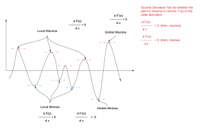
Substitute the value of x in the function and find the value where the function has either minimum values or maximum values. In order to find whether the point is local/global minima or maxima, take the second-order derivative and determine whether the value is positive or negative. If the second-order derivative value is positive, the point is local or global minima and if the second-order derivative value is negative, the point is local or global maxima. The diagram below represents the same.

You may want to check out my post on gradient descent to understand the importance of finding the minima of the function in the context of machine learning.
Conclusions
Here is the summary of what you learned about local minima and global minima of the function:
- A function can have multiple minima and maxima.
- The point where function takes the minimum value is called as global minima. Other points will be called as local minima. At all the minima points, the first order derivative will be zero and related value can be found where the local or global minima occurred.
- Similarly, the point where function takes the maximum value is called as global maxima. Other points will be called as local maxima.
- Local minima and global minima becomes important for machine learning loss or cost function.
- Completion Model vs Chat Model: Python Examples - June 30, 2024
- LLM Hosting Strategy, Options & Cost: Examples - June 30, 2024
- Application Architecture for LLM Applications: Examples - June 25, 2024
Leave a Reply