In this post, you will learn about how to train a Keras Convolution Neural Network (CNN) for image classification. Before going ahead and looking at the Python / Keras code examples and related concepts, you may want to check my post on Convolution Neural Network – Simply Explained in order to get a good understanding of CNN concepts.
Keras CNN Image Classification Code Example
First and foremost, we will need to get the image data for training the model. In this post, Keras CNN used for image classification uses the Kaggle Fashion MNIST dataset. Fashion-MNIST is a dataset of Zalando’s article images—consisting of a training set of 60,000 examples and a test set of 10,000 examples. Each example is a 28×28 grayscale image, associated with a label from 10 classes. Here is the code for loading the training data set after it is downloaded from Kaggle web page.
import pandas as pd
import numpy as np
from sklearn.model_selection import train_test_split
from keras import layers
from keras import models
from keras.utils import to_categorical
#
# Loading Fashion MNIST training and test dataset
#
fashion_mnist_train = pd.read_csv('/Users/apple/Downloads/archive/fashion-mnist_train.csv')
fashion_mnist_test = pd.read_csv('/Users/apple/Downloads/archive/fashion-mnist_test.csv')
#
# Examining the shape of the data set
#
fashion_mnist_train.shape, fashion_mnist_test.shape
Keras CNN model for image classification has following key design components:
- A set of convolution and max pooling layers
- A set of fully connected layers
- An output layer doing the classification
- Network configuration with optimizer, loss function and metric
- Preparing the training / test data for training
- Fitting the model and plot learning curve
CNN Design – Convolution & Maxpooling layers
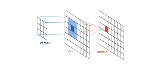
Designing convolution and maxpooling layer represents coming up with a set of layers termed as convolution and max pooling layer in which convolution and max pooling operations get performed respectively. Convolution operations requires designing a kernel function which can be envisaged to slide over the image 2-dimensional function resulting in several image transformations (convolutions). The kernel function can be understood as a neuron. And the different portions of image can be seen as the input to this neuron. Thus, there can be large number of points pertaining to different part of images which are input to the same / identical neuron (function) and the transformation is calculated as a result of convolution. The following image represents the convolution operation at a high level:
The output of convolution layer is fed into maxpooling layer which consists of neurons that takes the maximum of features coming from convolution layer neurons. The output in the max pooling layer is used to determine if a feature was present in a region of the previous layer. In simple words, max-pooling layers help in zoom out.
For Fashion MNIST dataset, there are two sets of convolution and max pooling layer designed to create convolution and max pooling operations. Here is the code for adding convolution and max pooling layer to the neural network instance. Note how the input shape of (28, 28, 1) is set in the first convolution layer. The first argument represents the number of neurons. Activation function used in the convolution layer is RELU.
#
# Setting up the convolution neural network with convnet and maxpooling layer
#
model = models.Sequential()
model.add(layers.Conv2D(32, (3, 3), activation='relu', input_shape=(28, 28, 1)))
model.add(layers.MaxPooling2D((2, 2)))
model.add(layers.Conv2D(64, (3, 3), activation='relu'))
model.add(layers.MaxPooling2D((2, 2)))
model.add(layers.Conv2D(64, (3, 3), activation='relu'))
#
# Model Summary
#
model.summary()
Executing the above code prints the following:
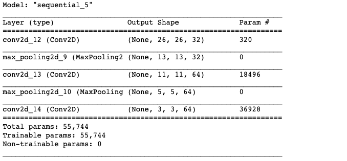
Note that the output of every Conv2D and Maxpooling2D is a 3D tensor of shape (hieight, width and channels). The width and height dimensions tend to shrink as you go deeper in the network. The number of channels is controlled by the first argument passed to the Conv2D layers.
CNN Design – Fully Connected / Dense Layers
Next step is to design a set of fully connected dense layers to which the output of convolution operations will be fed. The reason why the flattening layer needs to be added is this – the output of Conv2D layer is 3D tensor and the input to the dense connected requires 1D tensor. Thus, it is important to flatten the data from 3D tensor to 1D tensor. Also, note that the final layer represents a 10-way classification, using 10 outputs and a softmax activation. Here is the code representing the flattening and two fully connected layers.
#
# Adding the fully connected layers to CNN
#
model.add(layers.Flatten())
model.add(layers.Dense(64, activation='relu'))
model.add(layers.Dense(10, activation='softmax'))
#
# Printing model summary
#
model.summary()
CNN Design – Configuring Network for Training
In the next step, the neural network is configured with appropriate optimizer, loss function and a metric. Here is the code representing the network configuration. Note the usage of categorical_crossentropy as loss function owing to multi-class classification. Check out the details on cross entropy function in this post – Keras – Categorical Cross Entropy Function
#
# Configuring the network
#
model.compile(optimizer='rmsprop',
              loss='categorical_crossentropy',
              metrics=['accuracy'])
Prepare the Training, Validation and Test Dataset
We are almost ready for training. Lets prepare the training, validation and test dataset. We will set aside 30% of training data for validation purpose. Later, the test data will be used to assess model generalization. Note some of the following in the code given below:
- Training and validation data set is created out of training data
- Output label is converted using to_categorical in one-vs-many format.
- Data set is reshaped to represent the input shape (28, 28, 1)
- Data is converted into float type
Here is the code for creating training, validation and test data set.
#
# Preparing the training data set for training
#
X = np.array(fashion_mnist_train.iloc[:, 1:])
y = to_categorical(np.array(fashion_mnist_train.iloc[:, 0]))
#
# Create training and validation data split
#
X_train, X_val, y_train, y_val = train_test_split(X, y, test_size=0.3, random_state=42)
#
# Creating the test data set for testing
#
X_test = np.array(fashion_mnist_test.iloc[:, 1:])
y_test = to_categorical(np.array(fashion_mnist_test.iloc[:, 0]))
#
# Reshaping the dataset in (28, 28, 1) in order to feed into neural network
# Convnet takes the input tensors of shape (image_height, image_width, image_channels)
#
X_train = X_train.reshape(X_train.shape[0], 28, 28, 1)
X_test = X_test.reshape(X_test.shape[0], 28, 28, 1)
X_val = X_val.reshape(X_val.shape[0], 28, 28, 1)
#
# Changing the dataset to float
#
X_train = X_train.astype('float32')/255
X_val = X_val.astype('float32')/255
X_test = X_test.astype('float32')/255
#
# Examinging the shape of the dataset
#
X_train.shape, X_val.shape, X_test.shape
Fit the CNN Model and Plot the Learning Curve
Finally, lets fit the model and plot the learning curve to assess the accuracy and loss of training and validation data set. Here is the code. Note that epoch is set to 15 and batch size is 512.
#
# Fit the CNN model
#
history = model.fit(X_train, y_train,
                    validation_data=(X_val, y_val),
                    epochs=15,
                    batch_size=512)
The next step is to plot the learning curve and assess the loss and model accuracy vis-a-vis training and validation dataset. Here is the code:
import matplotlib.pyplot as plt

history_dict = history.history
loss_values = history_dict['loss']
val_loss_values = history_dict['val_loss']
accuracy = history_dict['accuracy']
val_accuracy = history_dict['val_accuracy']

epochs = range(1, len(loss_values) + 1)
fig, ax = plt.subplots(1, 2, figsize=(14, 6))
#
# Plot the model accuracy vs Epochs
#
ax[0].plot(epochs, accuracy, 'bo', label='Training accuracy')
ax[0].plot(epochs, val_accuracy, 'b', label='Validation accuracy')
ax[0].set_title('Training & Validation Accuracy', fontsize=16)
ax[0].set_xlabel('Epochs', fontsize=16)
ax[0].set_ylabel('Accuracy', fontsize=16)
ax[0].legend()
#
# Plot the loss vs Epochs
#
ax[1].plot(epochs, loss_values, 'bo', label='Training loss')
ax[1].plot(epochs, val_loss_values, 'b', label='Validation loss')
ax[1].set_title('Training & Validation Loss', fontsize=16)
ax[1].set_xlabel('Epochs', fontsize=16)
ax[1].set_ylabel('Loss', fontsize=16)
ax[1].legend()
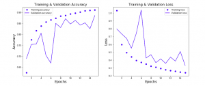
The following plot will be drawn as a result of execution of the above code:. Note that as the epochs increases the validation accuracy increases and the loss decreases.

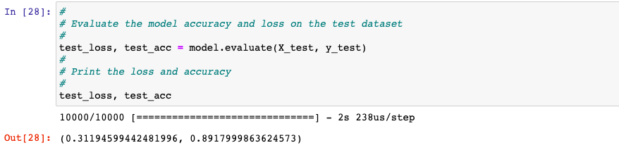
Finally, we will go ahead and find out the accuracy and loss on the test data set.
#
# Evaluate the model accuracy and loss on the test dataset
#
test_loss, test_acc = model.evaluate(X_test, y_test)
#
# Print the loss and accuracy
#
test_loss, test_acc
Conclusions
Here is the summary of what you have learned in this post in relation to training a CNN model for image classification using Keras:
- A set of convolution and max pooling layers would need to be defined
- A set of dense connected layers would need to be defined. There would be needed a layer to flatten the data input from Conv2D layer to fully connected layer
- The output will be 10 node layer doing multi-class classification with softmax activation function
- The shape of input data would need to be changed to match the shape of data which would be fed into ConvNet.
- Training, validation and test data can be created in order to train the model using 3-way hold out technique.
- The shape of training data would need to reshaped if the initial data is in the flatten format.

Check out my latest book titled as First Principles Thinking: Building winning products using first principles thinking.
- Three Approaches to Creating AI Agents: Code Examples - June 27, 2025
- What is Embodied AI? Explained with Examples - May 11, 2025
- Retrieval Augmented Generation (RAG) & LLM: Examples - February 15, 2025
I found it very helpful. However the differences are not too understandable for me