
In this post, you will learn about the concepts of Gradient Boosting Regression with the help of Python Sklearn code example. Gradient Boosting algorithm is one of the key boosting machine learning algorithms apart from AdaBoost and XGBoost.
What is Gradient Boosting Regression?
Gradient Boosting algorithm is used to generate an ensemble model by combining the weak learners or weak predictive models. Gradient boosting algorithm can be used to train models for both regression and classification problem. Gradient Boosting Regression algorithm is used to fit the model which predicts the continuous value.
Gradient boosting builds an additive mode by using multiple decision trees of fixed size as weak learners or weak predictive models. The parameter, n_estimators, decides the number of decision trees which will be used in the boosting stages. Gradient boosting differs from AdaBoost in the manner that decision stumps (one node & two leaves) are used in AdaBoost whereas decision trees of fixed size are used in Gradient Boosting.
The process of fitting the model starts with the constant such as mean value of the target values. In subsequent stages, the decision trees or the estimators are fitted to predict the negative gradients of the samples. The gradients are updated in the each iterator (for every subsequent estimators). A learning rate is used to shrink the outcome or the contribution from each subsequent trees or estimators.
In this post, you will learn about the concepts of gradient boosting regression algorithm along with Python Sklearn example.
GradientBoosting Regressor Sklearn Python Example
In this section, we will look at the Python codes to train a model using GradientBoostingRegressor to predict the Boston housing price. Sklearn Boston data set is used for illustration purpose. The Python code for the following is explained:
- Train the Gradient Boosting Regression model
- Determine the feature importance
- Assess the training and test deviance (loss)
Python Code for Training the Model
Here is the Python code for training the model using Boston dataset and Gradient Boosting Regressor algorithm. Note some of the following in the code given below:
- Sklearn Boston dataset is used for training
- Sklearn GradientBoostingRegressor implementation is used for fitting the model.
- Gradient boosting regression model creates a forest of 1000 trees with maximum depth of 3 and least square loss.
- The hyperparameters used for training the models are the following:
- n_estimators: Number of trees used for boosting
- max_depth: Maximum depth of the tree
- learning_rate: Rate by which outcome from each tree will be scaled or shrinked
- loss: Loss function to optimize. The options for the loss functions are: ls, lad, huber, quantile. ls represents least square loss. lad represents least absolute deviation. huber represents combination of both, ls and lad.
- Coefficient of determination, R-squared is used for measuring the model accuracy. The method score invoked on the instance of gradient boosting regression would result in printing the R-squared
- You can also calculate mean squared error (MSE) to measure the model performance.
from sklearn import datasets
from sklearn.preprocessing import StandardScaler
from sklearn.model_selection import train_test_split
from sklearn.pipeline import make_pipeline
from sklearn.ensemble import GradientBoostingRegressor
from sklearn.decomposition import PCA
from sklearn.metrics import mean_squared_error
#
# Load the Boston Dataset
#
bhp = datasets.load_boston()
#
# Create Training and Test Split
#
X_train, X_test, y_train, y_test = train_test_split(bhp.data, bhp.target, random_state=42, test_size=0.1)
#
# Standardize the dataset
#
sc = StandardScaler()
X_train_std = sc.fit_transform(X_train)
X_test_std = sc.transform(X_test)
#
# Hyperparameters for GradientBoostingRegressor
#
gbr_params = {'n_estimators': 1000,
          'max_depth': 3,
          'min_samples_split': 5,
          'learning_rate': 0.01,
          'loss': 'ls'}
#
# Create an instance of gradient boosting regressor
#
gbr = GradientBoostingRegressor(**gbr_params)
#
# Fit the model
#
gbr.fit(X_train_std, y_train)
#
# Print Coefficient of determination R^2
#
print("Model Accuracy: %.3f" % gbr.score(X_test_std, y_test))
#
# Create the mean squared error
#
mse = mean_squared_error(y_test, gbr.predict(X_test_std))
print("The mean squared error (MSE) on test set: {:.4f}".format(mse))
The model accuracy can be measured in terms of coefficient of determination, R2 (R-squared) or mean squared error (MSE). The model R2 value turned out to 0.905 and MSE value turned out to be 5.9486.
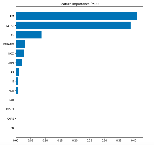
Determine the Features Importance
Here is the code to determine the feature important. Note the usage of attribute feature_importances_ to calculate the values of feature importances.
import numpy as np
import matplotlib.pyplot as plt
from sklearn.inspection import permutation_importance
#
# Get Feature importance data using feature_importances_ attribute
#
feature_importance = gbr.feature_importances_
sorted_idx = np.argsort(feature_importance)
pos = np.arange(sorted_idx.shape[0]) + .5
fig = plt.figure(figsize=(8, 8))
plt.barh(pos, feature_importance[sorted_idx], align='center')
plt.yticks(pos, np.array(bhp.feature_names)[sorted_idx])
plt.title('Feature Importance (MDI)')
result = permutation_importance(gbr, X_test_std, y_test, n_repeats=10,
                                random_state=42, n_jobs=2)
sorted_idx = result.importances_mean.argsort()
fig.tight_layout()
plt.show()
Here is how the plot would look like.
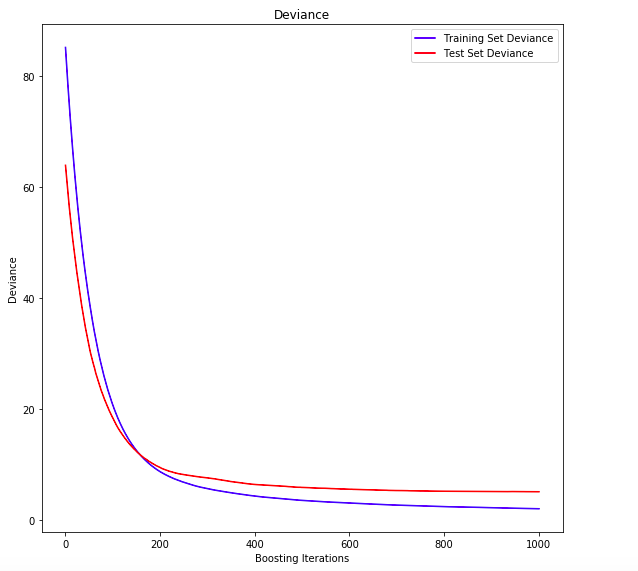
Assessing the Training & Test Deviance
Here is the Python code for assessing the training and test deviance (loss).
test_score = np.zeros((gbr_params['n_estimators'],), dtype=np.float64)
for i, y_pred in enumerate(gbr.staged_predict(X_test_std)):
    test_score[i] = gbr.loss_(y_test, y_pred)

fig = plt.figure(figsize=(8, 8))
plt.subplot(1, 1, 1)
plt.title('Deviance')
plt.plot(np.arange(gbr_params['n_estimators']) + 1, gbr.train_score_, 'b-',
         label='Training Set Deviance')
plt.plot(np.arange(gbr_params['n_estimators']) + 1, test_score, 'r-',
         label='Test Set Deviance')
plt.legend(loc='upper right')
plt.xlabel('Boosting Iterations')
plt.ylabel('Deviance')
fig.tight_layout()
plt.show()
Here is the plot representing training and test deviance (loss).
Here is a great Youtube video on Gradient Boosting Regression algorithm.
Conclusions
Here is the summary of what you learned in this post regarding the Gradient Boosting Regression:
- Gradient Boosting algorithm represents creation of forest of fixed number of decision trees which are called as weak learners or weak predictive models. These decision trees are of fixed size or depth.
- The gradient boosting starts with mean of target values and add the prediction / outcome / contribution from subsequent trees by shrinking it with what is called as learning rate.
- The decision trees or estimators are trained to predict the negative gradient of the data samples.
- Gradient Boosting Regression algorithm is used to fit the model which predicts the continuous value.

Check out my latest book titled as First Principles Thinking: Building winning products using first principles thinking.
- Three Approaches to Creating AI Agents: Code Examples - June 27, 2025
- What is Embodied AI? Explained with Examples - May 11, 2025
- Retrieval Augmented Generation (RAG) & LLM: Examples - February 15, 2025
I found it very helpful. However the differences are not too understandable for me