Linear Regression vs Logistic Regression: Python Examples

Last updated: 15th Dec, 2023

In the ever-evolving landscape of machine learning, two regression algorithms stand out for their simplicity and effectiveness: Linear Regression and Logistic Regression. But what exactly are these algorithms, and how do they differ from each other? At first glance, logistic regression and linear regression might seem very similar – after all, they share the word “regression.” However, the devil, as they say, is in the details. Each method is uniquely tailored to solve specific types of problems, and understanding these subtleties is key to unlocking their full potential.

Linear regression and logistic regression are both machine learning algorithms used for modeling relationships between variables but perform different tasks. Linear regression is used to model linear relationships and predict value of a continuous response variable, while logistic regression is used to model binary outcomes (i.e. whether or not an event happened) in form of predicting value of categorical response variable. In this blog post, we will discuss the differences between linear vs logistic regression, as well as when to use each one. We will also provide examples so that you can understand how they work.

What is Linear Regression?

Linear regression is a statistical method used in machine learning for predictive modeling. It models linear relationships between a continuous dependent variable and one or more independent variables including both categorical and continuous variables.

For example, let’s say we want to do predictive modeling around predicting house prices based on various features. Using a linear regression model, we can establish a relationship between the house price (dependent variable) and features like square footage, number of bedrooms, location, and age of the house (independent variables). The model will attempt to fit a linear equation to this data, enabling us to predict the price of a house given its characteristics.

Types of Linear Regression Models: Formula, Examples

Two common forms are simple linear regression (one independent variable) and multiple linear regression (two or more – multiple independent variables). The following are the formula and examples:

1. Simple Linear Regression: 

   • Formula of simple linear regression: y = β0 + βx. In the formula, y is the dependent variable, x is the independent variable, β0 is the intercept and β is the slope.
   • Example scenario: Predicting house prices based on size.
   • Independent or Predictor Variable: Size of the house (e.g., square feet). Note its just one independent variable.
   • Dependent or Response Variable: Price of the house.
   • Model: The price increases linearly with size. A line is fitted through data points representing house size and price, predicting price based on size.
   • When to use: Suitable when the goal is to predict the value of a dependent variable based on one independent variable. Simple linear regression model is often used as a starting point for analysis due to its simplicity and interpretability, even if later analyses involve more complex models.
     
     The following is the regression line plot representing the simple linear regression model discussed in this example:
     
     

2. Multiple Linear Regression:

   • Formula of multiple linear regression: y = β0 + β1×1+ β2×2+…+βnxn. In the formula, y is the dependent variable, x is the independent vector of independent variables, β0 is the intercept, and β1, β1, …, βn are coefficients for respective features such as x1, x2, …, xn.
   • Example scenario: Predicting a car’s fuel efficiency or house prices.
   • Independent or Predictor Variables: Engine size, weight of the car, year of manufacture. Note there are multiple independent variables.
   • Dependent or Response Variable: Miles per gallon (MPG).
   • Model: MPG is predicted based on a linear combination of engine size, weight, and year. The model accounts for how each factor affects MPG together.
   • When to use: When the goal is to understand the relationship between one dependent variable and two or more independent variables, multiple linear regression is appropriate. Multiple linear regression can handle both quantitative and categorical independent variables.

Loss function for linear regression models: Least Squares Method

The coefficients of best-fit linear regression models are learned using the least-squares method. The least-squares method is a mathematical procedure for finding the line of best fit for a set of data points. The cost function for linear regression is the sum of the squared residuals. The residual is the difference between the actual value and the predicted value. The gradient descent algorithm is used to find the line of best fit by minimizing the cost function.

Linear regression models are evaluated using R-squared and adjusted R-squared. R-squared represents the variation of the value of dependent variables which is explained by the linear regression model. The greater the value of R-squared, the better is the linear regression model. Adjusted R-squared is used when there are multiple independent variables in the linear regression model. It adjusts for the addition of variables and only increases if the new variable actually improves the model. Read further details in some of the following blogs:

• Linear regression model explained with real-world examples
• Linear regression hypothesis testing examples

Real-world examples of linear regression

Some of the real-world examples where linear regression models can be used are as follows:

• Predict the price of a house based on its size, number of bedrooms, number of bathrooms, etc.
• Predict the demand for a product based on advertising expenditure, price of the product, etc.
• Predict students’ grades based on hours spent studying, the difficulty level of the course, etc.
• Predict the stock price of a company based on its earnings per share, dividend per share, etc.
• Predict the number of taxi rides taken in a city based on weather conditions, time of the day, etc.

Training a Linear Regression model – Python Code

The following is the Python code used for training a linear regression model using the sklearn diabetes dataset.

from sklearn.datasets import load_diabetes
from sklearn.linear_model import LinearRegression
from sklearn.model_selection import train_test_split
from sklearn.metrics import mean_squared_error, r2_score

# Load the diabetes dataset
diabetes_data = load_diabetes()
X = diabetes_data.data
y = diabetes_data.target

# Splitting the data into training and testing sets
X_train, X_test, y_train, y_test = train_test_split(X, y, test_size=0.3, random_state=42)

# Create linear regression object
linear_regressor = LinearRegression()

# Train the model using the training sets
linear_regressor.fit(X_train, y_train)

# Make predictions using the testing set
y_pred = linear_regressor.predict(X_test)

# The coefficients
coefficients = linear_regressor.coef_
# The mean squared error
mse = mean_squared_error(y_test, y_pred)
# The coefficient of determination: 1 is perfect prediction
r2 = r2_score(y_test, y_pred)

coefficients, mse, r2

What is Logistic Regression?

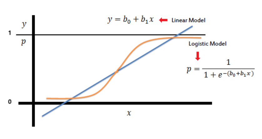
Logistic Regression is a statistical method used for analyzing datasets where one or more independent variables determine an outcome. This method is particularly useful in two main types of classification problems. First, in binary classification, where the outcome is a dichotomous variable with only two possible outcomes. Here, Logistic Regression is employed to predict the probability of a binary outcome, such as ‘yes’ or ‘no’, ‘success’ or ‘failure’, based on one or more predictor variables. Secondly, it extends to multinomial classification, which deals with scenarios where the outcome can fall into one of three or more categories. Read further details on this blog – Logistic regression explained with Python example

Key features of Logistic Regression

The following are some of the key features of logistic regression:

• Categorical Outcome: Logistic regression is ideal for predicting binary outcomes (e.g., success/failure, yes/no, 0/1).
• Probability Estimation: It estimates the probability that a given input point belongs to a certain class.
• Sigmoid Function: The core of logistic regression is the sigmoid (or logistic) function, which maps any real-valued number into a value between 0 and 1. The sigmoid function takes a linear combination of input features and maps it to output between 0 and 1. The logistic regression formula for the sigmoid function is:
  
  
  
  Here p(Y = 1) is the probability that the dependent variable Y = 1, X is the independent variable, β0​ is the intercept, and β1​ is the coefficient for X. The output of the sigmoid function represents the probability that an event will happen. If the probability is greater than 0.50, then the event is classified as “yes” or “true”. If the probability is less than 0.50, then the event is classified as “no” or “false”. The picture below represents a logistic regression model based on the sigmoid function.

Types of Logistic Regression Models

1. Binary Logistic Regression:
   • Formula: The basic formula is the logistic function as shown above.
   • Example: Predicting whether a student passes or fails an exam based on their hours of study.
2. Multinomial Logistic Regression:
   • Formula: This is used when the dependent variable has three or more nominal categories. The formula involves calculating probabilities of each category and using a softmax function.
   • Example: Classifying a set of fruits into categories like apples, oranges, and bananas based on features like weight, color, and diameter.
3. Ordinal Logistic Regression:
   • Formula: This is used for ordinal dependent variables where the categories are ordered. It uses thresholds to define the boundaries between ordered categories.
   • Example: Rating a restaurant experience as poor, average, good, or excellent.

How are Logistic Regression models evaluated?

Logistic regression models are evaluated using accuracy and the AUC-ROC curve. Accuracy represents the percentage of correctly predicted values (i.e. true positives + true negatives) out of all predicted values. In addition, other evaluation metrics such as precision, recall, and F-measure can also be used to evaluate the logistic regression model. The AUC-ROC curve is a graphical representation of how well the logistic regression model can discriminate between positive and negative outcomes. The greater the area under the curve, the better is the logistic regression model.

Loss Function for Logistic Regression Models: Cross Entropy Loss

In logistic regression, the cost function used to estimate the error of the model is the cross entropy loss, also known as log loss. It measures the performance of a classification model whose output is a probability value between 0 and 1. The loss increases as the predicted probability diverges from the actual label. The formula for cross entropy loss is (ylog(p) + (1 – y)log(1 – p)) , where y is the binary indicator (0 or 1) of the class label, and p is the predicted probability.

Real-world examples of Logistic Regression model

Some of the real-world examples where logistic regression models can be used are:

• Predict whether or not a customer will default on a loan
• Predict whether or not a patient will have a heart attack
• Predict whether or not an email is a spam
• Predict whether or not a student will pass/fail an exam

Training a Logistic Regression model – Python Code

The following Python code trains a logistic regression model using the IRIS dataset from scikit-learn. The model achieved an accuracy of 100% on the test set. This means that the logistic regression model was able to perfectly predict the species of all Iris flowers in the test set. This high level of accuracy is indicative of the distinctiveness of the features in the Iris dataset, which makes it relatively easier for classification models like logistic regression to perform well

from sklearn.datasets import load_iris
from sklearn.linear_model import LogisticRegression
from sklearn.model_selection import train_test_split
from sklearn.metrics import accuracy_score

# Load the Iris dataset
iris = load_iris()
X = iris.data
y = iris.target

# Splitting the data into training and testing sets
X_train, X_test, y_train, y_test = train_test_split(X, y, test_size=0.3, random_state=42)

# Create logistic regression object
logistic_regressor = LogisticRegression(max_iter=1000)

# Train the model using the training sets
logistic_regressor.fit(X_train, y_train)

# Make predictions using the testing set
y_pred = logistic_regressor.predict(X_test)

# The accuracy of the model
accuracy = accuracy_score(y_test, y_pred)
accuracy

Differences: Linear vs Logistic Regression

Having explored both linear and logistic regression, it’s clear that while they share some similarities, they are fundamentally different in several key aspects. The following is the list of differences between linear and logistic regression:

Aspect	Linear Regression	Logistic Regression
Dependent Variable	Continuous and unbounded (e.g., temperature, prices)	Categorical, often binary (e.g., yes/no outcomes)
Model Output	Continuous value (e.g., weight, salary)	Probabilities, mapped to classes (e.g., spam vs. not spam)
Use Case Scenarios	Predicting trends and outcomes in continuous data	Classification tasks, predicting likelihoods
Assumptions	Linearity, homoscedasticity, normal distribution of errors	No linear relationship required; binary/ordinal dependent variable
Result Interpretation	Coefficients represent change in dependent variable per unit change in independent variable	Coefficients used for odds ratios, indicating change in odds per unit change in independent variable

The choice between logistic and linear regression depends significantly on the data and the specific analytical question. Linear regression is more suited for modeling continuous outcomes, while logistic regression is preferred for classification and probability estimation tasks. Understanding these differences between logistic vs linear regression is crucial for effective model selection and achieving accurate predictions.