Gradient Descent in Machine Learning: Python Examples

Last updated: 22nd April, 2024

This post will teach you about the gradient descent algorithm and its importance in training machine learning models. For a data scientist, it is of utmost importance to get a good grasp on the concepts of gradient descent algorithm as it is widely used for optimizing/minimizing the objective function / loss function / cost function related to various machine learning models such as regression, neural network, etc. in terms of learning optimal weights/parameters. This algorithm is essential because it underpins many machine learning models, enabling them to learn from data by optimizing their performance. 

Introduction to Gradient Descent Algorithm

The gradient descent algorithm is an optimization algorithm used to minimize an objective function, commonly called the cost or loss function in machine learning. This cost function is a mathematical function used to calculate loss or error which is the difference between the model’s predicted value and the actual value in the real world for a given input data set. While training a model, the ask is to find a high-performance model (model with a minimal loss). To find the best model, we need to minimize the cost function. And, minimizing the cost function is about finding the most optimal values of parameters or weights vector that give the minimal loss for any given input data set. The algorithm used to minimize the cost function is called the gradient descent algorithm.

The term “gradient descent” is derived from two key concepts: “gradient” and “descent.”

1. Gradient: In mathematics and physics, the gradient of a function at any point is a multi-dimensional vector that points in the direction of the steepest increase of that function. The magnitude of the gradient vector at a point corresponds to the rate of greatest increase in the function’s value. In the context of a cost function in machine learning, the gradient indicates the direction in which the cost function rises most rapidly.
2. Descent: The word “descent” refers to the method’s objective of moving downwards to find the minima of the function. Since the gradient points toward the greatest increase, the opposite direction, in which the algorithm moves, will lead to the steepest decrease. By iteratively moving in the direction opposite to the gradient (hence “descending”), the algorithm finds the point where the cost or loss function attains its minimum value.

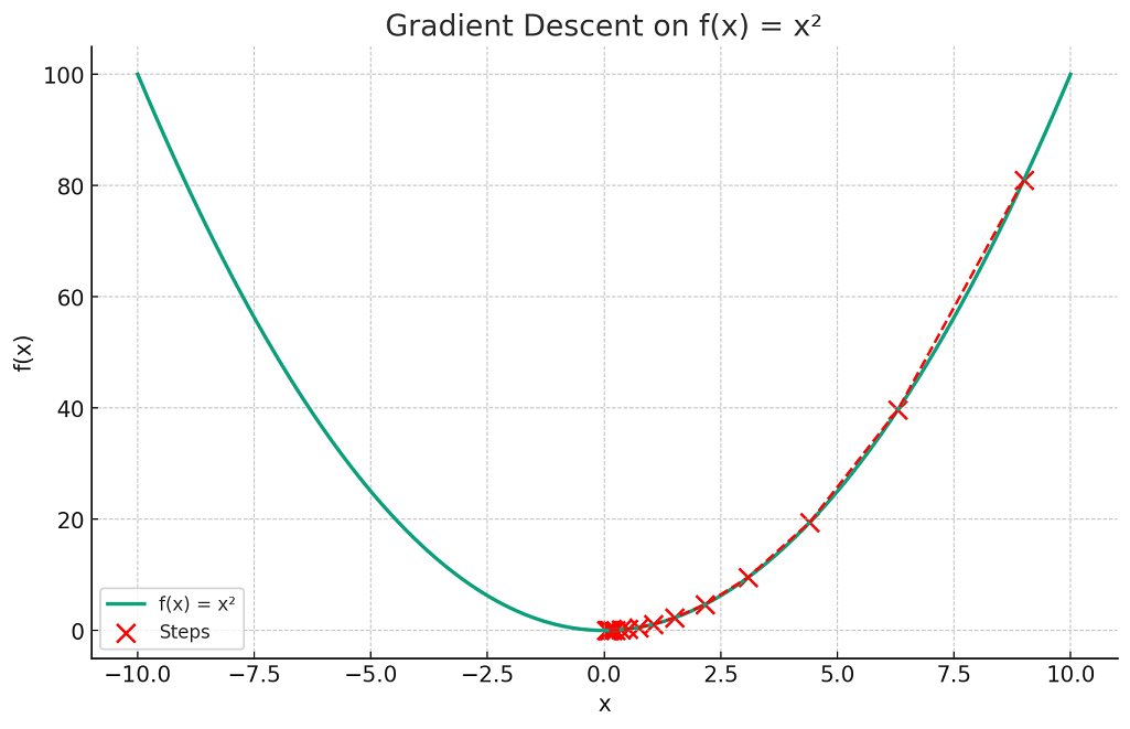
Thus, “gradient descent” is aptly named as it describes the process of descending (minimizing) a function by moving against (opposite to) its gradient. The following plot can be used to understand the gradient descent algorithm.

The plot visualizes the concept of gradient descent on a simple quadratic function f(x)=x2. The red dots represent the steps taken by the gradient descent algorithm starting from an initial point (here, x=9) and moving towards the minimum of the function at x=0.

Each step is determined by the gradient (slope) of the function at that point, and the algorithm iteratively moves in the direction that reduces the function’s value (i.e., descending). The red dashed line connects these steps, illustrating the path taken by the algorithm as it seeks the function’s minimum. This exemplifies how gradient descent navigates the function’s landscape to find the point of lowest value.

How to calculate Gradient Descent?

Calculating gradient descent involves several steps aimed at iteratively finding the minimum of a function. Here’s an expanded explanation with examples for better understanding:

1. Calculate the Gradient: The gradient is the derivative of the function with respect to different variables or parameters. In a simple one-dimensional case, if you have a function f(x), you calculate its derivative f′(x). For instance, if $f(x) = x^2$, then f′(x)=2x. In multi-dimensional scenarios, such as functions with multiple parameters (e.g., f(x,y)), you calculate the partial derivatives of each parameter.
2. Calculate Descent Value: The descent value is computed by multiplying the gradient by the learning rate (a small, positive number often less than 1). The learning rate determines the size of the algorithm’s steps toward reaching the function plot’s minimum point. For example, if the gradient at a point is 4 and the learning rate is 0.1, the descent value would be 0.1×4= 0.4.
3. Update the Parameters: The parameters of the function are updated by subtracting the descent value from their current values. This step is repeated iteratively. Continuing with the example above, if the current value of a parameter is 5, it would be updated to 5−(0.4)=4.6. This updating moves the parameter towards the function’s minimum. The following is the representation of the updation of parameters:
   
   
   
   In case of multiple parameters, the value of different parameters would need to be updated as given below:
   
   
   
4. Iterative Process: The process of calculating the gradient, descent value, and updating parameters is repeated until the changes become negligibly small or for a set number of iterations. This iterative process ensures that the algorithm moves towards the function’s minimum. The following is the representation using formula:
   
   
   
5. Example in a Real-World Scenario: Consider a machine learning model where you’re trying to minimize the error between predicted and actual values (the loss function). The parameters could be the weights in a linear regression model predicting house prices. The gradient descent algorithm would iteratively adjust these weights to minimize the difference (loss) between the predicted and actual house prices.
6. Visualization: Think of this process as a ball rolling down a hill. The ball represents the parameters, and the hill represents the function to be minimized. The ball rolls in the direction that takes it to the lowest point of the hill, which represents the minimum of the function.

Different Types of Gradient Descent Algorithms

Gradient descent algorithms could be implemented in the following two different ways:

Batch Gradient Descent

In batch gradient descent, the update of model parameters or weights is calculated using the entire training dataset at once. This means that for each step in the training process, the algorithm calculates the gradient of the cost function for the entire dataset. The idea is to find the overall direction of the cost function at each step.

This algorithm is often used when the training dataset is relatively small and can fit into memory comfortably. It’s also suitable for less complex models where the cost of computing the gradient for the whole dataset is not prohibitively high. For example, consider a linear regression model where you’re predicting housing prices based on features like size and location. If your dataset is small, you could use batch gradient descent to train your model, updating the weights based on the error calculated from the entire dataset.

Stochastic Gradient Descent (SGD)

Stochastic gradient descent updates the model’s parameters using only one training example or a small batch of examples at a time. This means the gradient and hence the parameter update is calculated and applied after each example or small batch, making the process more incremental.

SGD is particularly useful when dealing with large datasets that cannot fit into memory. It’s also favored when training complex models, as it can handle the high computational cost more efficiently. Additionally, the stochastic nature of SGD can help the model escape local minima, potentially leading to better solutions. For example, in a deep learning model for image classification with a massive dataset, using SGD would be practical. Here, the model parameters are updated incrementally as each image (or a small batch of images) is processed, enabling the model to learn progressively without the need to load the entire dataset into memory.

Gradient Descent Python Code Example

The following code represents the python code for implementing and plotting gradient descent algorithm:

import numpy as np
import matplotlib.pyplot as plt

# Defining a simple quadratic function and its derivative
f = lambda x: x**2
f_prime = lambda x: 2*x

# Generating values
x = np.linspace(-10, 10, 400)
y = f(x)

# Gradient descent settings
learning_rate = 0.15
x_start = 9  # Starting point
steps = [x_start]
n_iterations = 15

# Gradient Descent Iteration
for _ in range(n_iterations):
    x_start = x_start - learning_rate * f_prime(x_start)
    steps.append(x_start)

# Plotting the function
plt.figure(figsize=(10, 6))
plt.plot(x, y, lw=2, label="f(x) = x²")

# Plotting the steps
plt.scatter(steps, f(np.array(steps)), color='red', s=100, label='Steps')
plt.plot(steps, f(np.array(steps)), color='red', linestyle='--', lw=1.5)

# Annotations and labels
plt.title('Gradient Descent on f(x) = x²')
plt.xlabel('x')
plt.ylabel('f(x)')
plt.legend()
plt.grid(True)
plt.show()

Video on Gradient Descent Algorithm

Conclusion

As a summary, you learned the concepts of Gradient Descent along with some of the following aspects:

• The gradient descent algorithm is an optimization algorithm that is used to minimize the objective function. In case of machine learning, the objective function is called cost or loss function.
• The gradient of a function at any point can be calculated as the first-order derivative of that function at that point.
• In the case of multiple dimensions, the gradient of the function at any point can be calculated as the partial derivative of the function that points against different dimensions.
• Gradient descent represents the opposite direction of the gradient. The gradient of a function at any point represents the direction of the steepest ascent of the function at that point.
• Batch gradient descent represents updating the weights after all the training examples are processed. Stochastic gradient descent is about updating the weights based on each training data or a small group of training data.