Geometric Distribution Concepts, Formula, Examples

Geometric Distribution, a widely used concept in probability theory, is used to represent the probability of achieving success or failure in a series of independent trials, where the probability of success remains constant. It is one of the essential tools used in a wide range of fields, including economics, engineering, physics, and statistics. As data scientists / statisticians, it is of utmost important to understand its concepts and applications in a clear manner.

In this blog, we will introduce you to the basics of Geometric distribution, starting with its definition and properties. We will also explore the geometric distribution formula and how it is used to calculate the probability of success or failure in different scenarios. We will then provide some examples to help you understand the concept and apply it in real-world situations. Let’s dive in and explore the world of geometric distribution!

What is Geometric Distribution?

Geometric Distribution is a type of probability distribution which models the number of Bernoulli trials X which are required to get the first success.  It is defined by two parameters: the probability of success (p) and the number of trials (r). The probability distribution can be represented as P(X=r) which can be read as the probability that the value of X is r where r is number of trials needed to get the first success. The key point to note is that the “success” represents the occurrence of the event we are interested in. This essentially means that even if the event that we are interested in has negative connotations, it can still be considered as “success”. 

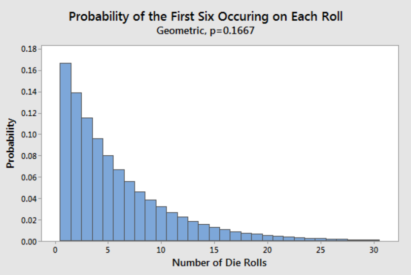
Let’s understand with a real-world example of tossing a dice. The random variable is number of trials it would take for 6 to arrive for the first time. P(X = 1) would represent the probability that 6 will show up on 1st trial. You could also calculate P(X=2), P(X=3), so on and so forth for calculating probability that 6 will occur on 2nd, 3rd trial respectively. The probability of success = 1/6 which can be calculated as 0.1667. You would want to note in the diagram below that probability is highest in the first trial and it decreases thereafter with each trial.

The following are necessary conditions for geometric distribution to happen:

• A series of independent trials can be run
• For each trial, there can be either success or failure. The probability of success remains same for each trial.
• The key thing is how many trials are needed in order to get the first successful outcome.

The geometric distribution can be used to model processes such as whether an event occurs within a certain period or not, patient recovery rate in medical science, etc. Three real world examples which could be represented using geometric distribution are:

• The chance of winning a game of lotto can be represented using geometric probability distribution. Each ticket contains 6 numbers, and the player must match all the numbers to win the jackpot prize. The probability of matching all 6 numbers is very low, so it follows a geometric probability distribution.
• The likelihood of discovering new oil fields can be described using geometric probability distribution. When exploring for new oil sites, companies will take core samples from different areas in order to identify potential sites for drilling for oil. The likelihood that each sample will lead to a new discovery follows a geometric probability distribution due to the high uncertainty of finding an appropriate site with each exploration attempt.
• The odds of receiving grants or other forms of financial aid for educational purposes can also be represented using geometric probability distribution. Depending on the number of applicants and quality of applications, there is no guarantee that one’s request will be successful – thus demonstrating a low probability and making it fit into a geometric probability distribution.

Geometric Distribution Formula

Here are some of key formulas for Geometric distribution given X represents the random variable that takes the value of r, r being the number of trials to get the first success. The p represents probability of success and q represents 1-p.

Probability that X will take value of r can be represented as the following:

[latex]P(X=r) = pq^{r-1}[/latex]

P(X > r) is the probability that more than r trials will be needed in order to get the first successful outcome. The formula looks like the following. The formula represents the fact that first r trials would have to fail for first successful to happen in more than r trials.

[latex]P(X>r) = q^r[/latex]

Based on the above, P(X ≤ r) represents the probability that r or fewer trials than r would be needed in order for there to be a successful outcome.

[latex]P(X>r) = 1 – q^r[/latex]

Expected number of trials before the success happens can be represented using the following:

[latex]Expectation, E(X) = \frac{1}{p}[/latex]

The variance of number of attempts can be represented as the following:

[latex]Variance, Var(X) = \frac{q}{p^2}[/latex]

Conclusion

The geometric distribution is a powerful tool in statistics and probability that allows us to understand the behavior of a certain series of events. It is used to describe the probability of an event (success) occurring after a certain number of attempts and can be used to calculate the probability of success after each attempt. In real-world scenarios, this type of probability distribution model can be used in many different fields such as engineering, finance, medicine, and more. Not only can it help us better understand the likelihood of success for any given project or process but it can also help us make decisions about potential investments and future projects. With its unique ability to model outcomes accurately, the geometric distribution has been widely applied in many different fields with great success.